Vector index structures help AI databases find similar embeddings without comparing every stored vector one by one. The main families are flat indexes, graph indexes, cluster-based indexes, hash-based indexes, and quantized indexes. Each family optimizes a different part of the search problem: exact recall, low-latency navigation, scalable partitioning, fast approximate bucketing, or memory reduction. The right choice depends on how much build time, query time, memory, and recall you can trade for the workload you are running.
This guide explains the major vector index families, what each one is designed to optimize, and how to reason about the practical trade-offs. By the end, you should be able to look at an AI database workload and make a more informed decision about whether you need exact search, approximate search, graph navigation, clustering, hashing, quantization, or a combination of several techniques.
Why Vector Indexes Exist
AI applications often store data as embeddings, which are numerical vectors that represent the meaning, similarity, or features of text, images, audio, code, or other objects. A retrieval system compares a query vector against stored vectors and returns the nearest neighbors according to a distance or similarity measure such as cosine similarity, inner product, or Euclidean distance. Without an index, the system has to score every vector for every query. That can be acceptable for small collections, but it becomes expensive as the number of vectors, dimensions, users, and queries grows.
A vector index is a data structure that makes nearest neighbor search faster or smaller, usually by accepting some trade-off. Some indexes preserve exact results but do not reduce the amount of work very much. Others reduce the search space aggressively but may miss a relevant neighbor. Still others compress vectors to fit more data in memory, which can improve speed while introducing approximation error.
This is why vector indexing is less about finding one universally best structure and more about choosing the structure that matches the workload. A search system for a small internal knowledge base may prioritize simplicity and exactness. A large retrieval-augmented generation system may need high recall with predictable latency. A billion-vector image search system may prioritize memory compression and disk-aware routing. The same query model can lead to different index choices depending on scale and constraints.
Once the purpose of indexing is clear, the next step is to understand the main index families. Each family takes a different view of the search problem: scan everything, navigate a graph, search only nearby clusters, hash vectors into candidate buckets, or store compressed representations.
The Main Vector Index Families
The most common vector index structures can be grouped into five broad families. Real AI databases often combine them, but separating them conceptually makes the trade-offs easier to understand. A graph index may use quantized vectors. A cluster index may rerank candidates with exact vectors. A compressed index may still use a graph or inverted file structure for routing. The family names describe the core strategy, not always the complete implementation.
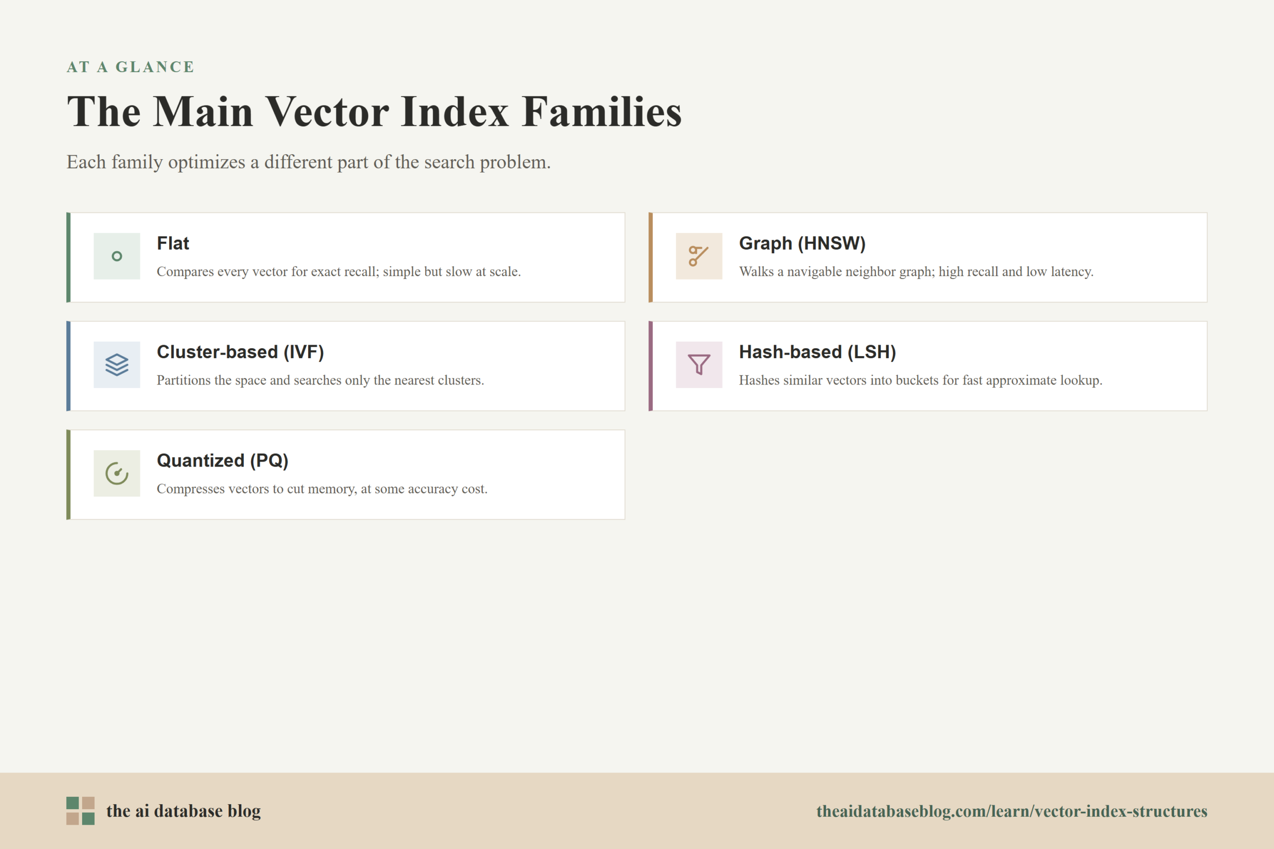
Flat Indexes
A flat index stores the original vectors and compares the query vector against every candidate vector. It is sometimes called brute-force search or exact nearest neighbor search. The word “index” can feel misleading here because a flat index does not avoid the full comparison in the way a tree, graph, or inverted structure does. Its value is that it provides exact results and a clean baseline for measuring approximate methods.
Flat search optimizes for recall and simplicity. If the vectors are stored in memory and the collection is small enough, flat search can be surprisingly competitive. It has no training step, no graph construction, no cluster assignment, and no search parameters that quietly change recall. It is also useful for evaluation because it can tell you what the true nearest neighbors are.
The cost is query time. A flat index has to compare the query with all stored vectors, so latency grows with the number of vectors. Memory use is also direct: storing 1 million 768-dimensional float32 vectors requires roughly 3 GB just for vector values before metadata and system overhead. Flat search can work well for small datasets, offline evaluation, high-precision reranking, or cases where only a small filtered subset is searched.
Graph Indexes
Graph indexes organize vectors as nodes connected to nearby vectors. During search, the system starts from one or more entry points and walks through the graph toward increasingly similar vectors. The best-known example is HNSW, short for Hierarchical Navigable Small World. Graph methods are popular because they often provide an excellent speed and recall balance for high-dimensional embedding search.
Graph indexes optimize for fast approximate retrieval with high recall. They do this by spending work during index construction to create useful neighbor links. At query time, the search follows those links rather than scanning the whole dataset. A wider or denser graph usually improves recall, but it also increases memory use and build cost.
The important trade-off knobs are usually build-time graph quality, graph density, and query-time exploration width. In HNSW-style indexes, a parameter such as M controls how many connections each vector can keep, a build parameter such as ef_construction controls how carefully neighbors are selected during construction, and a search parameter such as ef_search controls how many candidates are explored at query time. Higher values generally improve recall, but they also increase memory, build time, or query latency.
Graph indexes are often a strong default for AI database workloads where recall matters and the index can fit in memory. They are especially useful for semantic search and RAG systems where missing a relevant passage can reduce answer quality. Their weaker points are memory overhead, slower build time, and more complex behavior under heavy updates, deletes, or highly selective metadata filters.
Cluster-Based Indexes
Cluster-based indexes divide the vector space into groups, often using a coarse clustering method such as k-means. At query time, the system first finds the clusters closest to the query, then searches vectors inside only those clusters. In many systems this family is represented by inverted file indexes, often called IVF or IVFFlat when the vectors inside each cluster are stored without compression.
Cluster indexes optimize for narrowing the search space. Instead of asking, “Which of all vectors are closest?” the system first asks, “Which regions of the vector space should I inspect?” This can make search much faster on large datasets because only a subset of lists, partitions, or cells needs to be scanned.
The main build-time cost is training or choosing the cluster centers, then assigning vectors to those clusters. The main query-time knob is how many clusters to probe. Probing more clusters improves recall because the true nearest neighbor may not be inside the single closest cluster. Probing fewer clusters improves speed because fewer candidates are evaluated.
Cluster indexes can use less memory than graph indexes and can be easier to reason about for large datasets. They are also useful when a system benefits from partition-like behavior, such as searching only a few coarse regions or combining vector search with filtering strategies. Their challenge is that cluster boundaries are imperfect. If the data distribution is uneven, or if the query sits near a boundary between clusters, the best result may be in a list that is not searched unless the probe count is high enough.
Hash-Based Indexes
Hash-based vector indexes map vectors into buckets using functions designed to preserve some notion of similarity. The classic family is locality-sensitive hashing, often abbreviated as LSH. Similar vectors are more likely to land in the same bucket or share similar hash signatures, so the search system can inspect bucket candidates instead of the full dataset.
Hash indexes optimize for fast candidate generation and simple approximate lookup. They can be attractive when the search system needs lightweight routing, when binary signatures are useful, or when approximate recall is acceptable. Compared with graph and clustering methods, hash indexes are often easier to update because inserting a vector can mean computing its hash signature and placing it in one or more buckets.
The trade-off is that hashing can be blunt for modern dense embeddings. High-dimensional semantic vectors often need careful tuning, multiple hash tables, or longer signatures to avoid low recall. More hash tables or more bits can improve candidate quality, but they increase memory and lookup work. Fewer tables or shorter signatures reduce memory and query cost, but they may scatter genuinely similar vectors into different buckets.
Hash-based methods are less commonly the first choice for high-recall semantic search than graph or cluster indexes, but they remain important conceptually. They show one extreme of the indexing problem: use a cheap transformation to reduce the candidate set quickly, then accept that some nearby vectors may be missed unless the hash design is generous enough.
Quantized Indexes
Quantized indexes compress vectors or distance computations so that the system can store and search more data with less memory. Quantization can be used as a standalone compression strategy or combined with other index families. Common approaches include scalar quantization, product quantization, binary quantization, and residual quantization.
Quantization optimizes for memory efficiency, cache efficiency, and sometimes faster distance calculations. Instead of storing every dimension as a 32-bit floating point number, the system may store lower-precision values, compact codes, or compressed sub-vector representations. This can dramatically reduce memory use, which matters because many vector indexes are fastest when their working set fits in RAM.
The cost is approximation error. A compressed vector is not exactly the original vector, so distance estimates can be distorted. Systems often manage this by using quantized vectors for candidate generation and then reranking the final candidates with full-precision vectors. That hybrid pattern can preserve much of the memory benefit while recovering recall in the last step.
Quantization is especially important at large scale. If a collection is too large to fit comfortably in memory, reducing vector size may improve both cost and latency. However, aggressive quantization can reduce recall, especially when nearest neighbors are separated by small distance differences. The practical question is not whether compression changes results, but whether the recall loss is acceptable for the application.
These families are easier to compare when you look at what each one optimizes. The same terms appear repeatedly: build time, query time, memory, and recall. Understanding those four dimensions is the key to choosing an index without relying on vague labels like “fast” or “accurate.”
What Each Index Family Optimizes For
Every vector index makes a bet about where work should happen. Some structures do almost no work before queries and pay the cost during search. Others spend more time building a richer structure so that each query can be faster. Compression-based methods reduce memory pressure but may require extra reranking or careful tuning to maintain result quality. The best index is the one whose bet matches your system constraints.
| Index family | Primary optimization | Main cost | Typical use case |
|---|---|---|---|
| Flat | Exact recall and simplicity | Query time grows with dataset size | Small datasets, evaluation baselines, final reranking |
| Graph | High recall with low query latency | Memory overhead and build cost | Semantic search and RAG workloads where recall matters |
| Cluster | Reducing the search space by partitioning | Training, cluster tuning, and boundary misses | Large datasets where probing a subset is efficient |
| Hash | Fast approximate candidate bucketing | Recall sensitivity and possible need for multiple tables | Lightweight approximate lookup or binary signature workflows |
| Quantized | Lower memory use and compact computation | Approximation error and possible reranking complexity | Large-scale search, memory-constrained systems, compressed indexes |
Flat indexes optimize for truth. They are the simplest way to know whether an approximate index is missing results. Graph indexes optimize for navigability: they try to create shortcuts through the neighborhood structure of the data. Cluster indexes optimize for coarse routing: they try to avoid looking at regions that are unlikely to contain good matches. Hash indexes optimize for cheap bucketing. Quantized indexes optimize for smaller representations.
The important point is that these optimizations are not mutually exclusive. A system might use clustering to find candidate regions, product quantization to store compact codes inside those regions, and exact reranking for the top candidates. Another system might use a graph index over full vectors for high recall, then rely on metadata filtering and reranking downstream. Index families are building blocks, not fixed product categories.
After identifying what each family is trying to improve, the next practical question is how the four major trade-off dimensions interact. Build time, query time, memory, and recall are not independent. Improving one often pushes pressure onto another.
Build-Time Trade-Offs
Build time is the cost of creating the index before it can serve queries. It includes training cluster centers, assigning vectors, constructing graph connections, computing hash signatures, compressing vectors, and writing the resulting structure into memory or storage. Build time matters most when datasets are large, updates are frequent, or indexes need to be rebuilt regularly.
Flat indexes have almost no build-time complexity beyond storing vectors, which makes them useful when the dataset changes often or when the number of queries is too small to justify a complex index. Hash indexes can also be relatively cheap to build if the hash functions are fixed and insertion only requires computing signatures.
Graph indexes typically have higher build costs because the system must decide which neighbor links to create. Better construction settings can improve recall later, but the extra effort happens before query time. A graph built too cheaply may never reach the desired recall, even if query-time search is widened later, because the navigational structure itself is weaker.
Cluster indexes require a training or clustering phase. The number and quality of clusters matter because they determine how well the index can route queries. Too few clusters may leave each list too large, reducing speed. Too many clusters may increase training cost, memory overhead, and the chance that relevant neighbors are split across many lists.
Quantized indexes add training or encoding work depending on the method. Scalar quantization may be relatively straightforward. Product quantization and residual quantization can require learning codebooks and encoding vectors into compact representations. That build cost may be worthwhile if it allows a much larger working set to stay in memory.
Build time is often easy to underestimate because it is not visible in a single query benchmark. A system that looks fast after the index is built may still be expensive operationally if every major data refresh requires a long rebuild. That leads naturally to the next dimension: what the index does when users actually search.
Query-Time Trade-Offs
Query time is the latency and compute cost of finding nearest neighbors for one query or a batch of queries. It is where most users feel the effect of indexing. In AI applications, query latency can influence chat response time, recommendation freshness, agent workflow speed, and the number of retrieval calls a system can afford to make before generating an answer.
Flat search has predictable query behavior because it scores every vector. The downside is that the work grows linearly with the number of candidates. This makes flat search a good baseline but a poor fit for large, high-throughput retrieval unless the filtered candidate set is small or specialized hardware makes the scan acceptable.
Graph search usually provides low latency by exploring only a small part of the graph. The query-time exploration setting controls how wide the search is. A narrow search is faster but may stop before finding the best candidates. A wider search improves recall but increases latency. This is one reason graph indexes are useful in production: many systems can tune the search width per workload or even per query class.
Cluster search depends heavily on the number of clusters probed. Searching one or a few clusters is fast, but recall may suffer if relevant vectors are outside those clusters. Searching many clusters improves recall but moves the behavior closer to a larger scan. Cluster indexes are therefore best understood as a controlled way to choose how much of the dataset to inspect.
Hash search is fast when bucket candidates are small and meaningful. If buckets are too large, the system still has to scan many candidates. If buckets are too narrow, recall can drop. Multiple hash tables can improve the chance of finding similar items, but each table adds lookup and memory cost.
Quantized search can reduce query time when compressed vectors improve cache locality or enable faster approximate distance computations. However, if the system must rerank many candidates with original vectors to recover recall, the final latency depends on both the compressed search and the reranking stage.
Query speed alone does not tell the full story. A fast index that misses important results may harm the application more than it helps. That is why query-time tuning has to be evaluated alongside memory use and recall, rather than treated as a separate optimization problem.
Memory Trade-Offs
Memory is often the constraint that decides which vector index structures are practical. Embeddings are large, and many high-performance index structures are designed to keep most of their working set in RAM. Once the index no longer fits comfortably in memory, latency can become less predictable, costs can rise, and the system may need compression, sharding, disk-aware indexing, or a different retrieval architecture.
Flat indexes store the full vector data with little structural overhead. That can be memory-efficient in the sense that there is no graph or cluster structure layered on top, but the raw vectors themselves may still be large. A flat index over float32 embeddings becomes expensive as dimensions and row counts increase.
Graph indexes add memory for neighbor links. A denser graph improves navigability and recall, but those links are not free. This is why graph parameters affect both quality and memory. Higher connectivity can be valuable for difficult high-dimensional datasets, but it may be unnecessary or unaffordable for simpler workloads.
Cluster indexes usually add memory for centroids and list structures, but they can avoid the larger link overhead associated with graph indexes. If vectors inside the clusters are stored uncompressed, the raw vector memory remains the main cost. If clustering is combined with quantization, the memory footprint can fall substantially.
Hash indexes store signatures and bucket structures. Depending on the design, this can be compact, but multiple hash tables or long signatures can increase memory. Hashing also does not remove the need to store original vectors if exact reranking is required.
Quantized indexes are the main family built around memory reduction. By storing lower-precision values or compact codes, they can make large collections more practical. The risk is that too much compression can distort similarity. In many production-style systems, quantization works best when paired with a reranking stage that uses original or higher-precision vectors for the final top results.
Memory trade-offs are closely tied to recall because a smaller representation may be faster and cheaper, but it may also be less faithful to the original distances. That brings us to the quality dimension that matters most for most AI retrieval systems.
Recall Trade-Offs
Recall measures how many of the true nearest neighbors an index returns. In approximate nearest neighbor search, recall is rarely a simple yes-or-no property. It depends on the index family, parameters, dataset distribution, query type, filters, distance metric, and reranking strategy. For AI database workloads, recall is important because retrieved items often become the context for a downstream model.
Flat indexes provide exact nearest neighbors, so they are the recall baseline. If an approximate index returns the same top results as a flat search, recall is high. If it misses close neighbors that the flat search would have found, recall is lower. This is why teams often evaluate approximate indexes against a flat index on a sample dataset before choosing parameters.
Graph recall depends on graph quality and search width. A well-built graph with enough connectivity can reach high recall quickly. A sparse graph or narrow search may be fast but fragile. Some relevant vectors may be reachable only if the search explores enough candidate paths.
Cluster recall depends on whether the right clusters are probed. If a query’s true neighbors are concentrated in a few nearby clusters, the index can be both fast and accurate. If neighbors are scattered across boundaries, recall depends on probing more clusters. Metadata filtering can complicate this because the nearest vectors overall may not satisfy the filter, and the system may need to scan deeper to find enough valid results.
Hash recall depends on the probability that similar vectors share buckets or signatures. This probability is the heart of locality-sensitive hashing. The more aggressively the system narrows candidates, the more likely it is to miss some neighbors. More tables, longer searches, or broader candidate collection can improve recall at a cost.
Quantized recall depends on how much information is lost during compression. Light compression may have little practical effect, while aggressive compression can reorder close neighbors. Reranking can help because the index may only need to produce a good candidate set, not the final exact order.
Recall should be measured against the user experience, not just as an abstract benchmark. In a RAG system, the question is not only whether the mathematical nearest neighbor appears, but whether the retrieved context contains the facts needed to answer correctly. Still, mathematical recall is a useful starting point because it reveals whether the index is losing candidates before the rest of the retrieval pipeline can use them.
How To Choose A Vector Index Structure
Choosing a vector index is easiest when you start with the workload rather than the algorithm. The same index can behave differently depending on dataset size, vector dimensionality, update rate, metadata filters, latency budget, hardware, and acceptable recall loss. A good selection process asks what the application cannot compromise on, then chooses the simplest index that satisfies that constraint.
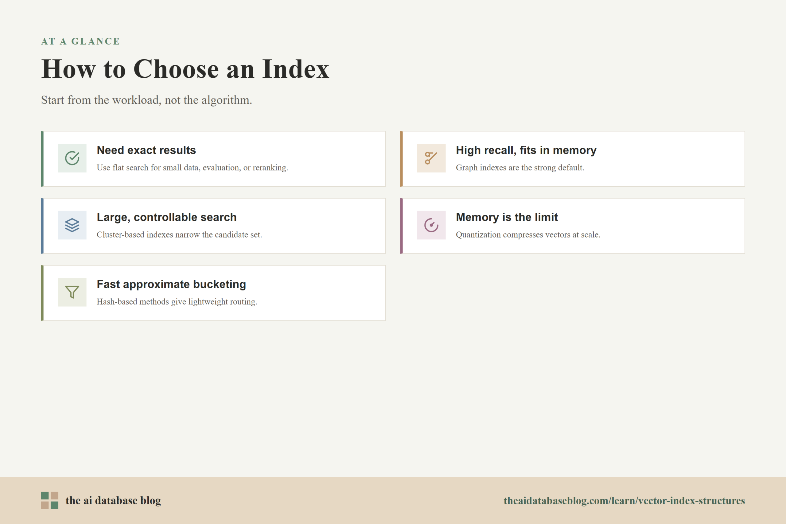
If exact results matter more than speed, start with flat search. This is common for small datasets, evaluation, or final reranking. Flat search also helps you establish a recall baseline before tuning approximate indexes.
If you need high recall and low latency on a dataset that can fit in memory, graph indexes are often the first serious candidate. They are strong for semantic search and many RAG workloads because they can retrieve good candidates quickly without scanning most of the corpus. Tune build quality and query exploration carefully, because default parameters may not match your data.
If your dataset is large and you want a controllable way to reduce the candidate set, cluster-based indexes are a practical option. They are especially useful when memory is a concern, when build cost needs to be lower than a dense graph, or when probing a subset of partitions gives a good enough recall and latency curve.
If memory is the limiting factor, consider quantization. Compression can be used with graph or cluster indexes, and it often becomes more important as collections move from millions to hundreds of millions or billions of vectors. Test the compression level against recall because the right answer depends on how separable your embeddings are.
If the workload needs fast approximate bucketing, binary signatures, or a lightweight candidate generator, hash-based methods may be useful. They are usually not the default for high-recall dense semantic search, but they can still be valuable in specialized retrieval architectures.
A practical way to compare options is to run a small benchmark with your own data. Measure exact recall using flat search, then test approximate indexes across several parameter settings. Track build time, query latency, memory footprint, recall, filtered-query behavior, and update cost. The best index is the one that lands on the right curve for your application, not the one that wins a generic benchmark.
Common Hybrid Patterns
Many production retrieval systems do not rely on a single pure index family. They combine routing, compression, filtering, and reranking to get a better overall balance. This is important because the initial vector index is only one part of retrieval. The system may also apply metadata filters, keyword search, business rules, diversification, cross-encoder reranking, or generation-time context selection.
One common pattern is approximate candidate generation followed by exact reranking. A graph, cluster, hash, or quantized index returns a larger candidate set than the final result count. The system then recomputes distances using full-precision vectors or applies a more expensive ranking model to the candidates. This helps recover quality while keeping the first-stage search fast.
Another pattern is cluster routing with quantized storage. The index first finds relevant partitions, then searches compressed vectors inside those partitions. This can be useful when memory is tight and the system needs to search very large collections. The final results may be reranked with original vectors if they are available.
Graph plus quantization is also common. The graph provides navigable structure, while quantized vectors reduce memory or speed up distance calculations. The trade-off is that graph quality and compressed-distance quality both affect recall, so evaluation becomes more important.
Filtered retrieval adds another layer. A vector index may return nearest neighbors that do not satisfy metadata conditions such as tenant, category, language, access permission, or timestamp. If filtering happens after approximate search, the system may need to search deeper to find enough valid results. In some cases, exact search over a small filtered subset or partition-aware indexing can outperform a generic approximate index.
These hybrid patterns reinforce the main lesson: index choice is part of retrieval architecture. The best structure is not only the one with the fastest nearest neighbor search, but the one that works well with filters, updates, memory limits, reranking, and the downstream AI task.
Mental Model For The Trade-Offs
A simple mental model is to treat vector indexing as a budget allocation problem. You have a limited budget for build time, query time, memory, and recall loss. Flat indexes spend very little build complexity but pay heavily at query time. Graph indexes spend build time and memory to reduce query time while preserving high recall. Cluster indexes spend training and routing complexity to scan fewer vectors. Hash indexes spend recall risk to get cheap buckets. Quantized indexes spend precision to save memory.
If you increase recall, you usually pay somewhere. A graph search may explore more candidates. A cluster search may probe more lists. A hash search may use more tables. A quantized system may rerank more candidates with full vectors. If you reduce memory, you may accept more approximation or more complicated reranking. If you reduce build time, you may get a weaker structure and slower or less accurate queries.
This does not mean every trade-off is painful. Good tuning can improve both speed and recall compared with poor defaults. Better filtering strategy can reduce wasted search. Quantization can improve latency if it keeps the working set in memory. But there is usually no free index setting that maximizes everything at once.
The most reliable approach is to choose a baseline, measure, and then move one constraint at a time. Start with flat search for truth. Try a graph index if latency is too high and memory is available. Try clustering if scale or memory pushes against graph overhead. Add quantization when memory becomes the bottleneck. Consider hashing for specialized approximate bucketing. Evaluate each step against the actual retrieval task.
FAQs
1.
1. What is the difference between exact and approximate vector search?
Exact vector search returns the true nearest neighbors according to the chosen distance metric, usually by comparing the query against all candidate vectors. Approximate vector search uses an index structure to avoid some comparisons, which makes search faster or smaller but may miss some true nearest neighbors. Flat indexes are exact, while graph, cluster, hash, and quantized indexes usually involve approximation unless configured to search exhaustively.
2.
2. Why are graph indexes so common in AI databases?
Graph indexes are common because they often deliver high recall with low query latency for dense embeddings. They create neighbor links between vectors so the search can navigate toward good matches instead of scanning the entire dataset. Their main drawback is that the graph consumes memory and can take longer to build than simpler index structures.
3.
3. When should I use a flat vector index?
Use a flat index when the dataset is small enough for direct search, when you need exact results, or when you need a baseline for evaluating approximate indexes. Flat search is also useful as a final reranking step after an approximate index has produced a manageable candidate set.
4.
4. How do cluster-based indexes affect recall?
Cluster-based indexes affect recall by deciding which clusters are searched for each query. If the true nearest neighbors are inside the probed clusters, recall can be high. If relevant vectors are in clusters that were not probed, the index can miss them. Increasing the number of probed clusters usually improves recall but also increases query time.
5.
5. Does quantization always reduce search quality?
Quantization introduces approximation, so it can reduce search quality if compression changes the distance relationships between vectors. However, the practical effect depends on the compression method, dataset, and reranking strategy. Many systems use quantized vectors for fast candidate generation and then rerank with higher-precision vectors to recover quality.
6.
6. Which vector index is best for RAG?
For many RAG systems, a graph index is a strong starting point because it can provide high recall at low latency. However, the best choice depends on corpus size, memory budget, update rate, metadata filters, and the cost of missing relevant context. Smaller systems may use flat search, larger systems may use clustering or quantization, and mature systems often combine approximate search with reranking.
Takeaway
Vector index structures are different ways of spending build time, query time, memory, and recall. Flat indexes give exact results and a useful baseline, graph indexes offer strong low-latency recall when memory allows, cluster indexes reduce the search space through coarse routing, hash indexes provide lightweight approximate bucketing, and quantized indexes make large collections more memory-efficient. This guidance is most useful for engineers, architects, and technical product teams designing AI database systems, especially retrieval systems for semantic search or RAG, where the practical goal is not simply to pick the fastest index but to choose the structure that returns good enough context within the system’s latency and cost limits.