AI databases are built around one core job: storing data in a form that can be searched by meaning, not only by exact keywords or fixed fields. Internally, they combine a storage engine, vector indexes, metadata indexes, query execution logic, filtering, replication, sharding, compaction, and operational controls. The hardest engineering work is not simply finding similar vectors quickly. It is balancing relevance, latency, freshness, memory use, disk cost, filtering accuracy, and scale as data and query traffic grow.
This guide explains the main internal components of an AI database and how they work together. You will learn how vectors and metadata are stored, why different index structures exist, how queries are executed, why filtering changes search behavior, how systems scale across machines, and what trade-offs engineers make when designing databases for retrieval-augmented generation, semantic search, recommendation, and other AI applications.
What Makes an AI Database Different From a Traditional Database?
An AI database still has many recognizable database concerns: it must store records, accept writes, serve reads, recover from failures, apply access rules, and expose query APIs. The difference is that one of its most important data types is the embedding, which is a high-dimensional vector representation of meaning. Instead of asking only for records where a field equals a value, an application may ask for records whose vector is closest to a query vector.
That changes the internal architecture. A traditional database can often use B-tree indexes, hash indexes, columnar layouts, or inverted indexes to narrow down exact matches and ranges. An AI database also needs a similarity search layer that can compare vectors efficiently. A direct comparison against every vector is simple but too slow for large datasets, so the database usually builds an approximate nearest neighbor index, often called an ANN index.
The database also has to connect vector search with ordinary structured constraints. A user may search for semantically similar support tickets, but only within one customer account, one language, one product line, and a date range. This is why AI databases are not just vector search libraries wrapped in an API. They are full data systems that combine vector search with persistence, metadata filtering, query planning, durability, scaling, and operational management.
Once that distinction is clear, the next question is where the data actually lives and how the database keeps it usable as writes, deletes, and updates arrive over time.
The Storage Engine
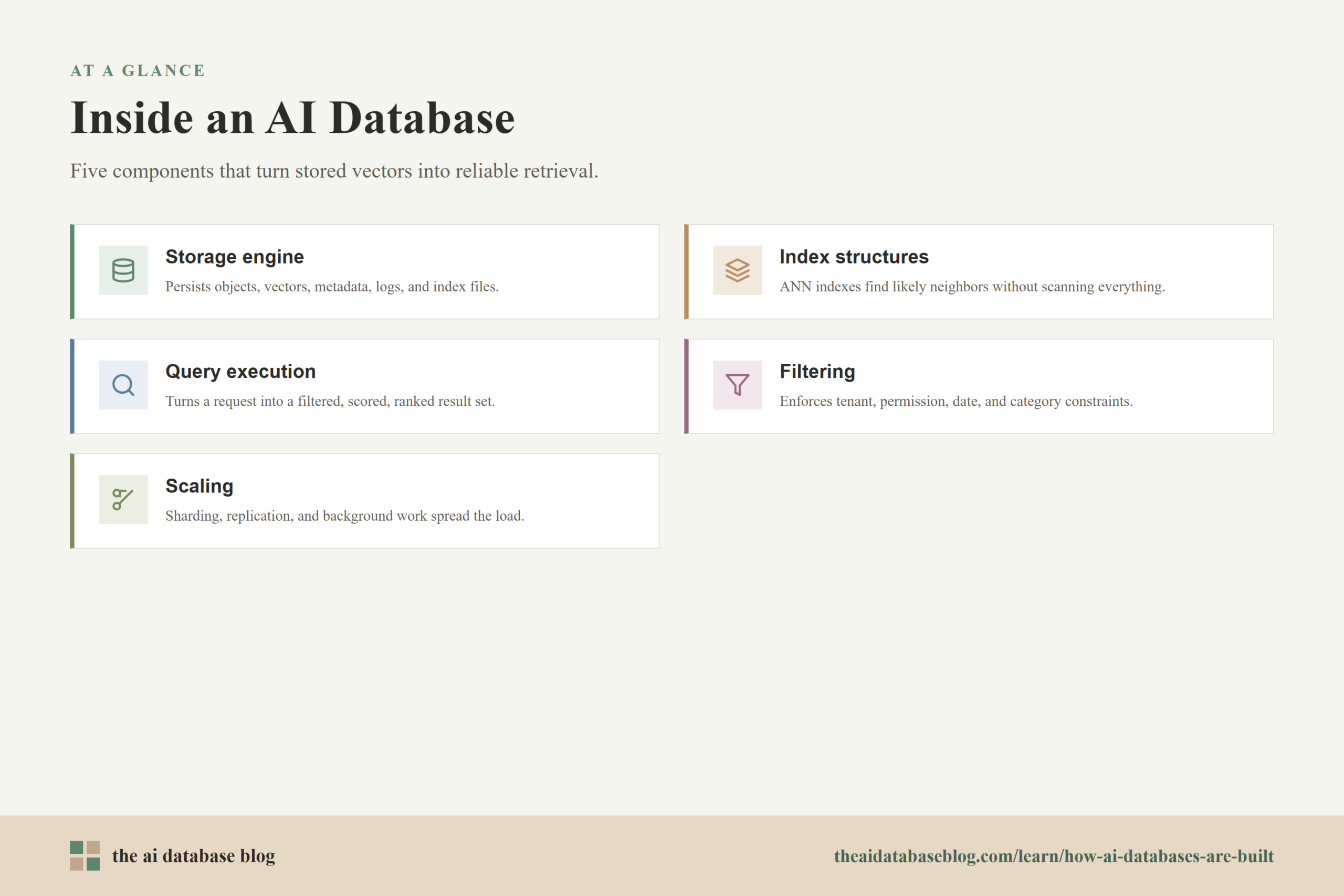
The storage engine is the part of an AI database responsible for persisting objects, vectors, metadata, and internal index files. It decides how data is written to disk, how it is flushed from memory, how deletes are tracked, how segments are compacted, and how the system recovers after a restart. In practice, the storage engine has to serve two different needs at the same time: fast ingestion for new or updated records, and fast retrieval for queries that need stable, searchable indexes.
Objects, Vectors, and Metadata
Most AI database records contain at least three pieces: the original object or document reference, one or more embeddings, and metadata fields. The object may be a text chunk, product record, image reference, support ticket, or document passage. The embedding is the numeric representation used for similarity search. The metadata is structured information such as tenant ID, timestamp, source, language, category, permissions, or status.
Good storage design keeps these pieces connected without forcing every query to read everything. A vector search may need the embedding and object ID first, then fetch the full object only for the final results. A filtered query may need metadata before or during vector traversal. A reranking step may need text or additional fields after the candidate set is selected. Separating these access patterns helps reduce unnecessary disk and memory work.
Write-Ahead Logs, Segments, and Compaction
Many AI databases use storage patterns similar to log-structured systems. New writes are appended to a durable log so they can be recovered after failure. Data is then organized into segments or partitions that can be indexed and searched. Over time, smaller segments may be merged into larger ones through compaction, which reduces the number of files and indexes a query must touch.
This design is useful because vector indexes can be expensive to update. Some index structures handle incremental inserts well, while others work best when built in batches. Segment-based storage lets the database accept new data quickly while building or rebuilding indexes in the background. The trade-off is freshness versus efficiency: if the system makes every new vector searchable immediately, query-time work may rise; if it batches too aggressively, newly written data may take longer to appear in search results.
Memory, Disk, and Cache Layout
AI databases must decide which data belongs in memory and which can stay on disk. Keeping full vectors and graph indexes in memory can make queries fast, but memory becomes expensive at large scale. Disk-based systems reduce memory pressure by storing more data on SSDs and keeping only routing structures, compressed vectors, or hot portions of the index in memory.
The storage layer therefore affects query performance directly. If a query needs many random disk reads, latency rises. If compressed vectors are used, memory cost falls but exact distance estimates may become less precise. If full vectors are fetched only for final reranking, the system can keep candidate generation fast while still improving final result quality.
Storage choices set the boundaries for indexing. The index determines which records are considered likely matches, but the storage engine determines how expensive it is to maintain and read those records. That is why index design is the next major piece of the architecture.
Index Structures
Index structures are the data structures that let an AI database find likely nearest neighbors without comparing the query to every stored vector. No single index is best for every workload. The right design depends on dataset size, dimensionality, update rate, memory budget, recall target, filter selectivity, and latency requirements. Most production systems expose tuning options because a small change in index parameters can shift the balance between speed and accuracy.
Flat Indexes
A flat index compares the query vector against every stored vector. It is simple, exact, and useful for small collections or evaluation because it can provide ground-truth results. Its weakness is that search time grows with the number of vectors. At large scale, exact scanning becomes too expensive unless the system can use specialized hardware, aggressive partitioning, or a small candidate set.
Graph Indexes
Graph indexes connect vectors to nearby vectors, creating a navigable structure. At query time, the system starts from one or more entry points and traverses the graph toward closer candidates. Hierarchical graph approaches such as HNSW add layers so the search can move quickly through coarse neighborhoods before refining results in denser lower layers.
Graph indexes are popular because they can provide strong recall and low latency for many high-dimensional workloads. Their main trade-off is memory. The graph needs to store vectors or compressed representations plus edges between nearby points. More edges can improve recall, but they also increase memory use and build cost. Updates can also be more complex than appending to a simple list because new points need meaningful graph connections.
Cluster and Partition Indexes
Cluster-based indexes group vectors into partitions, often using centroids that represent regions of the vector space. During search, the database finds the most relevant partitions and scans or searches only within those partitions. Inverted file indexes, often called IVF indexes, follow this general idea.
This approach can reduce query work substantially because the database does not need to visit every vector or every shard. It can also make disk and cache behavior more predictable when similar vectors are stored near each other. The trade-off is that clustering introduces boundary errors: a true nearest neighbor may live in a partition the query did not visit. Increasing the number of partitions searched can improve recall, but it also increases latency.
Quantized and Disk-Based Indexes
Quantization compresses vectors so they take less memory or disk space. Product quantization, scalar quantization, binary quantization, and other compression methods reduce cost, but they also approximate the original vector values. Many systems use compressed vectors for candidate generation and fetch full-precision vectors later for reranking.
Disk-based indexes are designed for datasets that are too large to keep fully in memory. They typically keep a smaller routing structure or compressed representation in memory while storing larger graph or vector data on SSDs. This can make billion-scale search more affordable, but it raises new engineering concerns around disk layout, random reads, prefetching, caching, and update cost.
Indexes decide where the database searches, but they do not decide the whole query path. A real query also has filters, limits, scoring rules, hybrid text matching, authorization constraints, and result assembly. Those responsibilities belong to query execution.
Query Execution
Query execution is the process that turns an application request into a ranked result set. In an AI database, this usually means receiving a query vector or generating one, applying filters, selecting indexes or partitions, searching candidate vectors, merging partial results, optionally reranking, and fetching the final objects. The query executor is where database behavior becomes visible to the application: latency, result quality, and consistency all meet here.
From Query Request to Candidate Set
A vector query begins with a query embedding. Sometimes the application supplies the vector directly. In other cases, the database or surrounding retrieval system creates the embedding from text, image, or another input. The query executor then chooses the relevant collection, tenant, shard, partition, and index. If the system is distributed, it may send the query to multiple nodes and later merge their local top results.
The first output is usually a candidate set, not the final answer. Candidate generation is optimized for speed and recall. It tries to find enough likely matches so that the best results are included, even if the initial ordering is not perfect. The candidate set may be larger than the requested final result count because later stages need room to apply reranking, permissions, or additional filters.
Distance Metrics and Scoring
Vector search depends on a distance or similarity function. Common choices include cosine similarity, dot product, and Euclidean distance. The right metric depends on how the embeddings were produced and normalized. A database must store enough index metadata to interpret scores correctly, and it must avoid mixing incompatible vectors or metrics in the same search path.
Scores are often useful for ranking but not always meaningful as absolute values. A cosine score in one embedding model may not be comparable to a score from another model. This matters when a system combines multiple vector fields, merges text and vector search, or uses thresholds to decide whether a result is good enough for retrieval-augmented generation.
Hybrid Search and Reranking
Many AI applications use hybrid search, which combines vector similarity with lexical search. Vector search is good at semantic matching, while lexical search is good at exact terms, identifiers, rare names, and domain-specific phrases. A hybrid executor must combine signals from different indexes and normalize their scores in a useful way.
Reranking is another common stage. The database or retrieval pipeline may take the top candidates and apply a more expensive model or exact scoring function to reorder them. This can improve relevance, but it adds latency and compute cost. The engineering question is how many candidates to rerank: too few may miss better answers, while too many may slow the system down.
Query execution becomes harder when filters enter the picture. Filters sound simple because traditional databases handle them every day, but filters can interfere with approximate vector search in ways that are not obvious at first.
Filtering
Filtering is the part of an AI database that limits search results by structured conditions. A filter might require documents from a specific tenant, products in stock, records created after a certain date, or content a user has permission to access. In AI databases, filtering is not an optional convenience. It is often required for correctness, security, and relevance.
Pre-Filtering
Pre-filtering applies structured constraints before vector search. The database first narrows the searchable set, then runs similarity search within that subset. This can be accurate and efficient when the filtered subset is small and well indexed. It can also be difficult if the vector index was built for the full dataset and does not support efficient traversal inside arbitrary filtered subsets.
For example, if a user asks for only documents from one tenant, pre-filtering can prevent the system from searching unrelated data. But if the tenant has very few vectors, a graph index built across all tenants may not have enough useful connections inside that filtered subset. The search may need special entry points, filter-aware graph traversal, or a fallback scan.
Post-Filtering
Post-filtering runs vector search first, then removes results that do not match the filter. This is simple to implement and works well when filters are broad. The problem appears when filters are selective. If only one percent of the data matches the filter, most of the top vector candidates may be discarded, and the final result set may be too small or low quality.
Systems can compensate by retrieving more candidates before applying the filter, but that raises query cost. If the filter is extremely selective, retrieving more candidates may still fail because the approximate search path was never guided toward the filtered portion of the data.
Filter-Aware Indexing
Filter-aware indexing tries to make structured constraints part of the search strategy. The database may maintain inverted indexes for metadata, partition data by common filter keys, use bitmaps to represent matching object sets, choose entry points that satisfy filters, or prune graph traversal based on attribute constraints. Recent research on filtered ANN search shows that design choices such as pruning strategy, entry point selection, and filter selectivity can strongly affect performance.
The practical lesson is that metadata filtering should be treated as a first-class architecture concern. A database that performs well on unfiltered vector search may behave very differently when most production queries include tenant, permission, category, or time filters.
Filtering shows why single-node performance is only part of the story. Once data grows beyond one machine, the database also has to decide how to divide work across nodes while preserving relevance and predictable latency.
Scaling and Distributed Architecture
Scaling an AI database means handling more vectors, more writes, more queries, larger tenants, stricter latency targets, and higher availability requirements. The system can scale vertically by using larger machines with more memory, faster disks, or specialized accelerators. It can also scale horizontally by spreading data and query work across many machines. Horizontal scaling is powerful, but it adds query routing, result merging, replication, rebalancing, and failure handling.
Sharding
Sharding divides data across multiple partitions or nodes. A simple approach is hash-based sharding, where records are distributed by ID or tenant. This is operationally straightforward because writes are easy to route and shards can be balanced by size. The query cost is that a vector search may need to fan out to many shards, search each local index, and merge the partial top results.
Another approach is semantic or global partitioning, where vectors are assigned to partitions based on location in vector space. This can reduce query fanout because the database searches the partitions most likely to contain nearby vectors. The trade-off is operational complexity. The system must train or maintain a global partitioning structure, handle shifting data distributions, and rebalance partitions without harming freshness or availability.
Replication and Availability
Replication keeps copies of data on multiple nodes so the system can survive failures and serve more read traffic. Replication improves availability, but it raises questions about consistency and freshness. If a write is acknowledged before every replica has indexed it, a query may see different results depending on which replica serves it. If the system waits for all replicas, writes become slower.
AI databases often choose different consistency behavior depending on workload. A production search application may tolerate slight indexing delay if availability and latency remain strong. A compliance or permission-sensitive workload may require stricter guarantees around metadata updates and deletes. Architecture has to reflect which kind of correctness matters most.
Background Work
Large AI databases do a lot of work outside the foreground query path. They build indexes, compact segments, remove deleted records, refresh caches, rebalance shards, replicate data, and update statistics for query planning. This work must be scheduled carefully. If background compaction consumes too many resources, query latency suffers. If it runs too slowly, queries may touch too many small segments and become inefficient.
At scale, the database is not only a search algorithm. It is a continuously operating system that must coordinate ingestion, indexing, storage cleanup, and query serving without letting one activity starve the others.
The internal pieces now fit together: storage preserves and organizes data, indexes reduce search work, query execution coordinates retrieval, filtering enforces structured constraints, and scaling distributes the workload. The final design depends on which trade-offs the system chooses.
Engineering Trade-Offs
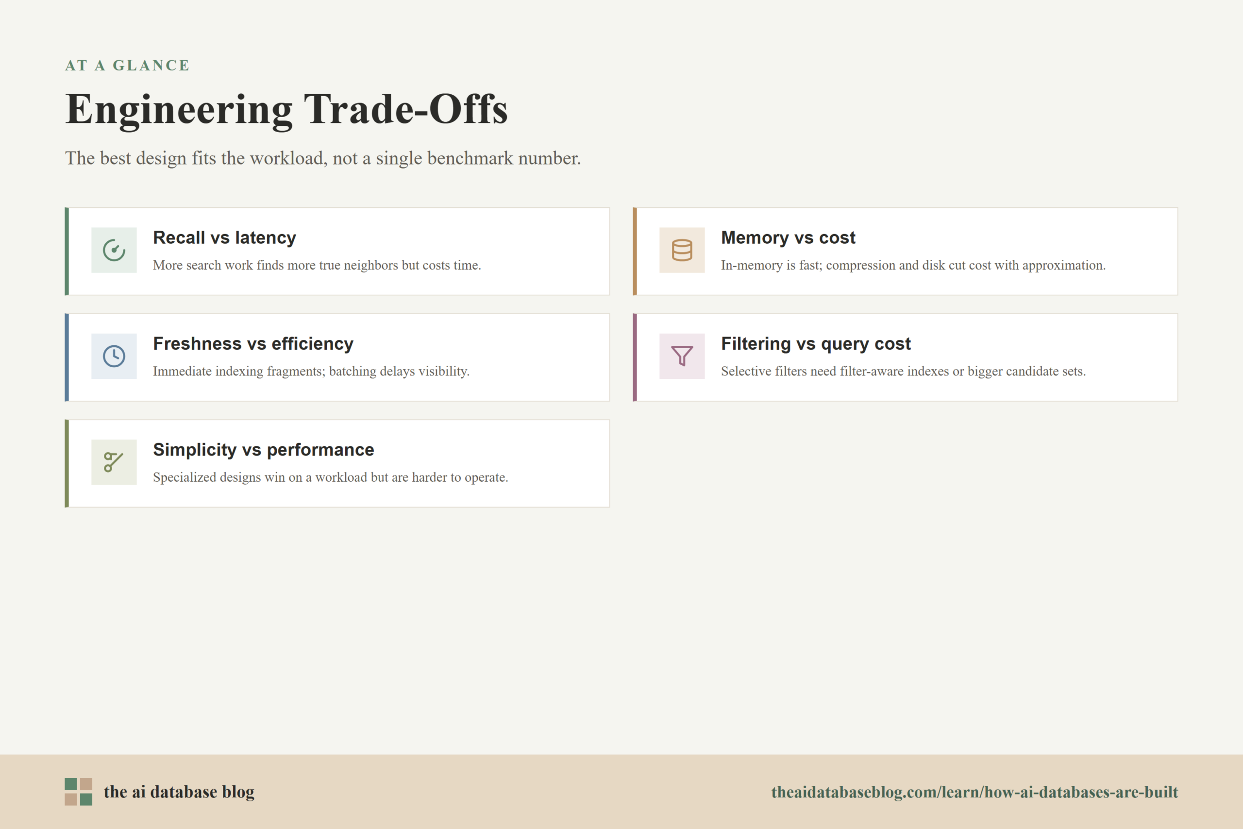
Every AI database architecture is a set of trade-offs. The best design is not the one that maximizes a single benchmark number. It is the one that fits the workload, data distribution, operational budget, and relevance requirements. Engineers usually tune these systems by measuring recall, latency, throughput, memory, disk use, build time, update speed, and failure behavior together.
Recall Versus Latency
Recall measures how many of the true nearest neighbors the system finds. Higher recall usually requires more search work: visiting more graph nodes, probing more partitions, scanning more candidates, or reranking a larger set. Lower latency usually requires doing less work. The tuning challenge is to find the point where result quality is good enough for the application without wasting compute on unnecessary precision.
Memory Versus Cost
Keeping indexes and vectors in memory can deliver fast search, but memory is expensive. Compression, disk-based indexing, and partitioning reduce memory requirements, but they introduce approximation, disk access, or routing overhead. A small semantic search application may be happiest with a memory-heavy graph index. A billion-vector system may need disk-aware layouts and compressed candidate generation.
Freshness Versus Index Efficiency
Freshness describes how quickly new or changed data becomes searchable. Immediate indexing is attractive for user-facing applications, but it can make writes expensive and create fragmented indexes. Batch indexing and compaction are more efficient, but they delay visibility. Many systems use a layered approach: a fresh mutable segment for recent writes plus optimized immutable segments for older data.
Filtering Accuracy Versus Query Cost
Strict filters are essential for many workloads, especially multi-tenant and permission-aware retrieval. But selective filters can make approximate search less efficient. The database may need metadata indexes, partition-aware routing, filter-aware traversal, or larger candidate sets. Each option improves correctness or recall in filtered queries but adds storage, memory, or query complexity.
Simplicity Versus Specialized Performance
A simpler architecture is easier to operate, debug, and scale predictably. A specialized architecture can produce better performance for a specific workload, but it may be harder to tune and adapt. For example, local sharding is simple, but it may require broad fanout. Global vector partitioning can reduce search work, but it requires more coordination and careful handling of changing data distributions.
These trade-offs are easier to evaluate when they are tied to real use cases. Retrieval-augmented generation, semantic product search, image retrieval, and recommendation systems all use similar building blocks, but they often prioritize different outcomes.
Architecture Articles Hub
The architecture of an AI database is easier to understand when each component has its own focused explanation. Use this hub to connect readers to deeper Architecture articles that explain the main parts of the system in more detail. The links below are structured as internal-link placeholders because the exact live Architecture URLs should be verified against the site sitemap before publication.
- Storage Engine Architecture: how AI databases persist vectors, objects, metadata, logs, segments, and deletes.
- Index Structures: how flat, graph, cluster, quantized, and disk-based indexes support similarity search.
- Query Execution: how vector queries move from request to candidate generation, scoring, reranking, and result assembly.
- Filtering Architecture: how metadata filters, permissions, and structured constraints interact with approximate nearest neighbor search.
- Scaling AI Databases: how sharding, partitioning, replication, routing, and background work support larger workloads.
- Engineering Trade-Offs: how teams balance recall, latency, memory, disk cost, freshness, and operational complexity.
A hub is most useful when it helps readers move from the big picture to the specific component they are trying to understand. After the internal URLs are added, this section can serve as the central entry point for the Architecture cluster.
FAQs
1. Is an AI database the same thing as a vector database?
Not always. A vector database is usually focused on storing embeddings and running similarity search. An AI database may include vector search, but it can also include hybrid retrieval, metadata filtering, document storage, permissions, reranking, and operational features that support AI applications. In practice, the terms often overlap, but AI database is the broader architectural idea.
2. Why do AI databases use approximate nearest neighbor search?
They use approximate nearest neighbor search because exact comparison against every vector becomes expensive as datasets grow. ANN indexes reduce the amount of work needed to find likely matches. The trade-off is that the system may not always return the mathematically exact nearest neighbors, so engineers tune the index to balance recall and latency.
3. What is the hardest part of building an AI database?
The hardest part is usually not one component in isolation. It is making storage, indexing, filtering, query execution, and scaling work together under real workloads. A design that performs well for unfiltered vector search may struggle with selective metadata filters, frequent updates, multi-tenant isolation, or strict freshness requirements.
4. How does filtering affect vector search?
Filtering changes which vectors are allowed to appear in the result set. If the filter is broad, the database may search normally and remove a few nonmatching results. If the filter is selective, the database may need filter-aware indexes, metadata bitmaps, special graph traversal, or larger candidate sets to avoid missing relevant results.
5. Why not keep every vector index in memory?
Keeping everything in memory can be fast, but it becomes costly as datasets grow. Large vector collections may require disk-based indexes, compressed vectors, partitioning, or tiered storage. These approaches reduce memory cost, but they introduce trade-offs around latency, recall, update speed, and disk access patterns.
6. How should teams evaluate AI database architecture?
Teams should evaluate architecture against their own workload rather than relying only on generic benchmarks. Important measurements include recall, latency, throughput, memory use, disk use, ingestion speed, update freshness, filtered query performance, failure recovery, and operational complexity. The right architecture depends on which constraints matter most for the application.
Takeaway
AI databases are built by combining storage engines, vector indexes, metadata filtering, query execution, and distributed systems engineering into one retrieval platform. This guidance is most useful for engineers, architects, and technical decision-makers who need to understand why AI database behavior changes across workloads. For a retrieval-augmented generation system, for example, the best architecture is not simply the fastest vector index; it is the design that returns relevant, permission-safe, fresh results within the application’s latency and cost limits.