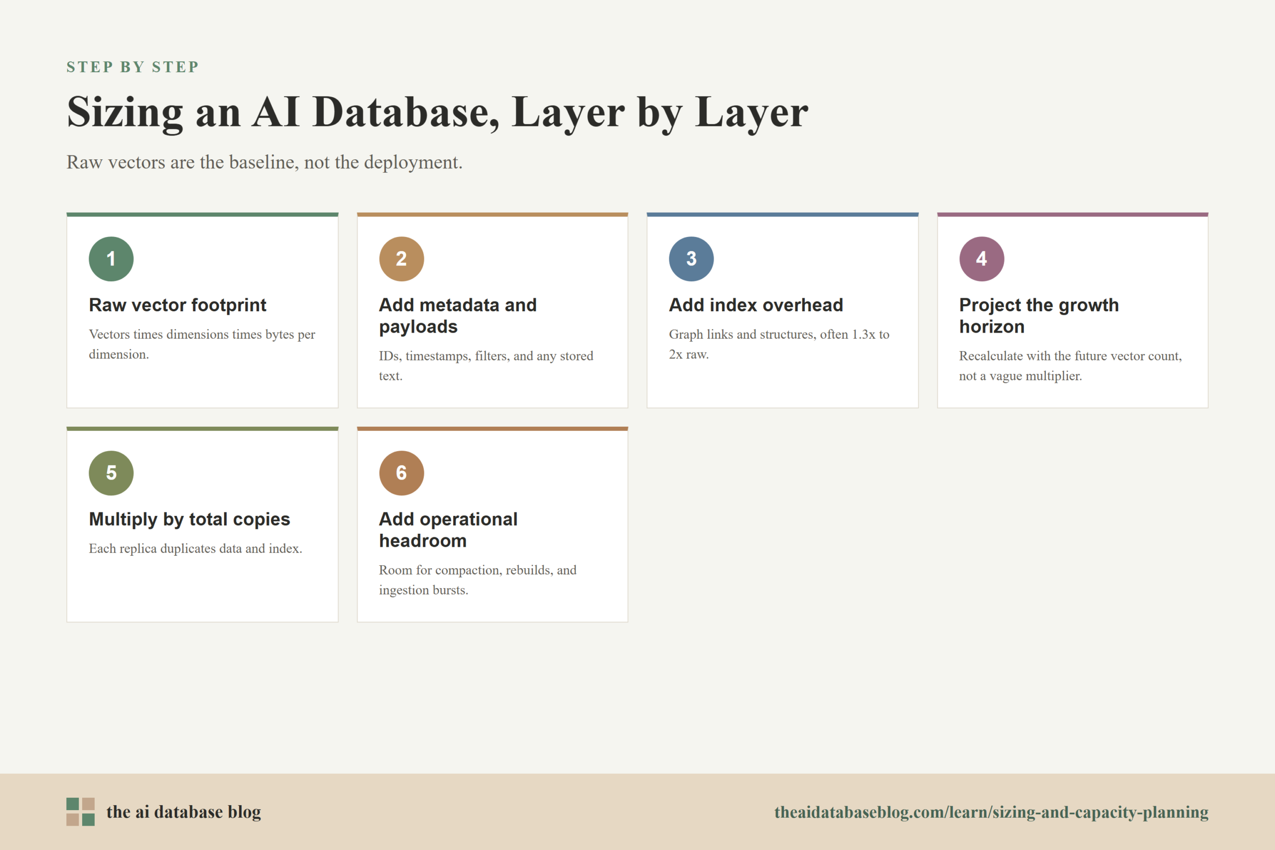
Sizing an AI database starts with a simple estimate: vector count multiplied by vector dimension multiplied by bytes per dimension. That gives the raw vector footprint, but it is only the baseline. A production plan also needs room for index structures, metadata, write overhead, replicas, backups, growth, and temporary space during ingestion or index rebuilds. The safest approach is to calculate the raw data size first, apply a realistic index and operational overhead factor, then multiply by the number of replicas and expected growth window.
This guide explains how to estimate memory and storage from vector count and dimension, why index headroom matters, and how to plan for future growth and replicas without overbuilding blindly. By the end, you should be able to make a practical first-pass capacity estimate, understand the assumptions behind it, and know which variables to validate before moving from a prototype to a production deployment.
Why Capacity Planning Matters for AI Databases
AI databases store and search embeddings, which are numeric representations of text, images, audio, code, or other data. These embeddings are usually high-dimensional vectors, and each vector can consume much more space than a traditional identifier or keyword field. When an application grows from thousands of records to millions or billions, vector storage and index memory can become one of the largest infrastructure costs in the retrieval system.
Capacity planning matters because vector search performance is closely tied to how much data must be held in memory, cached efficiently, or accessed from fast storage. If the system is undersized, queries may become slower, ingestion may fail, or index rebuilds may compete with live traffic. If the system is oversized, the application may carry unnecessary memory, storage, and replication costs before the workload needs them.
A good sizing plan does not try to predict every future detail perfectly. Instead, it separates the known quantities from the uncertain ones. Vector count, dimension, data type, metadata size, index type, replication factor, and expected growth rate can each be estimated, measured, and revised as the system matures.
Once the main sizing inputs are clear, the next step is to convert them into a baseline. That baseline is the raw vector footprint, which is the easiest part of the calculation and the foundation for everything that follows.
Estimate Raw Vector Memory and Storage
The raw vector footprint is the amount of space needed to store the vectors themselves before adding index structures, metadata, replicas, logs, or backups. It is determined by three values: the number of vectors, the number of dimensions in each vector, and the number of bytes used to store each dimension. This calculation is simple, but it is important because every later estimate builds on it.
The basic formula is:
Raw vector bytes = vector count x dimensions x bytes per dimension
For many embedding workloads, vectors are stored as 32-bit floating point values. A 32-bit float uses 4 bytes per dimension. If a system stores 10 million vectors with 768 dimensions each, the raw vector calculation is 10,000,000 x 768 x 4 bytes, which equals 30,720,000,000 bytes, or roughly 30.7 GB before binary-to-decimal conversion differences and system overhead.
Here are common byte assumptions:
- Float32: 4 bytes per dimension. This is a common default and a conservative starting point when no compression or quantization is assumed.
- Float16 or bfloat16: 2 bytes per dimension. This can reduce raw vector storage, but it should be tested for retrieval quality and system compatibility.
- Int8 or other quantized formats: 1 byte per dimension or less in some implementations. This can significantly reduce memory and storage, but it may affect recall, ranking quality, or re-ranking requirements.
Dimension has a direct and linear impact on capacity. If the vector count stays the same, moving from 768 dimensions to 1,536 dimensions roughly doubles the raw vector footprint. Likewise, doubling the number of stored objects doubles the raw footprint. This is why embedding model choice, chunking strategy, and deduplication all matter for infrastructure planning, not just retrieval quality.
Raw vector size is the cleanest number in the sizing process, but it is not the number to provision against. AI databases also store identifiers, metadata, inverted structures for filtering, write-ahead data, deleted or superseded records, and the index structures that make approximate nearest neighbor search fast. The next step is to add those layers without pretending the raw vector estimate is the whole system.
Add Metadata, Payloads, and Operational Storage
Most AI database records contain more than a vector. They usually include a stable object ID, source references, timestamps, tenant or access-control fields, document identifiers, chunk text, category fields, and other metadata used for filtering or display. Some systems store the original text payload alongside the vector, while others store only references to a separate document store. This design choice can change storage requirements dramatically.
Metadata is often smaller than the vector for high-dimensional embeddings, but it should not be ignored. A record with a 768-dimensional float32 vector uses about 3 KB for the raw vector alone. If the same record also stores 1 KB of text, IDs, and filterable attributes, metadata adds a meaningful amount to the total footprint. If the application stores long text chunks or large JSON payloads inside the database, payload storage can exceed the vector size.
Operational storage also includes data that is not always visible in a simple record schema. Databases may keep segment files, write-ahead logs, tombstones for deleted objects, compaction space, snapshots, and temporary files during index construction. These are normal parts of keeping a searchable system reliable, but they mean that disk planning should include more than the steady-state record size.
A practical first-pass storage estimate often looks like this:
- Raw vector storage: vector count x dimensions x bytes per dimension.
- Metadata and payload storage: average non-vector bytes per record x vector count.
- Index storage: an overhead factor based on the index type and parameters.
- Operational storage: extra room for logs, compaction, snapshots, temporary files, and rebuilds.
This broader estimate is more useful than raw vector storage alone because it reflects how the database is actually operated. It also prepares the next question: how much extra space is needed for the search index itself, especially when the index is optimized for low-latency approximate nearest neighbor search.
Plan Headroom for the Vector Index
The vector index is the structure that lets the database find similar vectors without comparing the query against every stored vector. Exact search may be feasible for small datasets, but many production systems use approximate nearest neighbor indexes to reduce latency at larger scale. These indexes improve query speed, but they require additional memory and storage beyond the raw vector data.
One common index family is HNSW, which organizes vectors into a graph. The database stores the vector data and additional graph connections that help searches move quickly toward nearby vectors. The memory overhead depends on index parameters, implementation details, and the number of links maintained per vector. As a rough planning range, an HNSW-style index is often estimated at about 1.3x to 2x the raw vector size before metadata and operational overhead, but the right factor should be confirmed with the specific database, index settings, and workload.
Index parameters change the tradeoff between memory, build time, recall, and latency. Higher connectivity can improve search quality or speed at query time, but it usually increases memory and build cost. Higher construction settings can improve the quality of the graph, but may require more CPU and temporary resources during indexing. These tradeoffs are why index headroom should be treated as a real capacity line item, not a small rounding error.
Headroom is also needed because indexes are not always built once and left unchanged forever. Production systems ingest new data, delete stale objects, update embeddings, compact segments, and rebuild or optimize indexes over time. During these operations, the system may temporarily need more memory, CPU, or disk than the final steady-state index requires.
A practical approach is to separate steady-state index overhead from operational headroom. Steady-state overhead covers the index that serves queries day to day. Operational headroom covers ingestion bursts, rebuilds, compaction, background merges, and unexpected growth. For many teams, planning at least 20% to 30% free capacity after expected steady-state usage is a useful starting point, with more headroom for fast-growing or write-heavy systems.
After index overhead is included, the estimate begins to look like a real deployment rather than a raw data calculation. The next adjustment is replication, because production systems usually need more than one copy of the data to support availability, durability, and read throughput.
Account for Replicas and Availability
Replicas are additional copies of data and indexes used to improve availability, durability, or read capacity. A single copy may be acceptable for a prototype, but production retrieval systems often need at least one additional replica so the application can continue serving queries during maintenance or node failure. Replicas can also help distribute query load when traffic grows.
From a capacity perspective, replicas are straightforward but easy to underestimate. If one complete copy of the vector data, metadata, and index requires 500 GB of usable capacity, then two replicas require roughly 1 TB before adding backup space, temporary operational headroom, or storage efficiency differences. Memory requirements can also multiply if each replica keeps its own in-memory index or cache.
The formula is:
Total replicated footprint = single-copy footprint x replica count
The term “replica count” should be defined carefully. Some teams use it to mean total copies, while others use it to mean extra copies in addition to the primary. For capacity planning, always write the calculation in terms of total copies. A primary plus one replica means two total copies. A primary plus two replicas means three total copies.
Replication also affects growth planning. If the dataset grows by 100 GB per month and the system keeps three total copies, the replicated footprint grows by about 300 GB per month before considering backups or temporary space. This multiplication is one reason to revisit retention rules, deduplication, chunking, and archival policies before simply adding more nodes.
Replicas help with resilience, but they are not the only way a vector database grows. Sharding, partitioning, and lifecycle policies also affect capacity because they determine where data lives, how queries fan out, and how much unused space is needed per node.
Plan for Growth, Shards, and Lifecycle Changes
Growth planning is not just a matter of adding a percentage to today’s dataset. AI database workloads can grow through new users, more source documents, finer chunking, additional embedding models, more tenants, or retained historical versions. Each growth path affects capacity differently. A system that doubles its document count behaves differently from one that keeps the same documents but stores embeddings from two models at once.
The first growth estimate should define a planning horizon. For example, a team might size for the next 6 months of expected growth plus enough free space to handle ingestion spikes and index maintenance. A longer horizon may be appropriate when procurement is slow or infrastructure changes require coordination. A shorter horizon may be better for early-stage systems where workload patterns are still changing quickly.
Sharding becomes important when one node cannot efficiently hold or search the full dataset. A shard is a portion of the data assigned to a node or partition. Sharding can improve capacity and parallelism, but it introduces query routing, coordination, and balancing concerns. If each query must search many shards, latency and network overhead may rise. If filters can route queries to a smaller subset of shards, the system can scale more efficiently.
Lifecycle planning can reduce capacity pressure before scaling becomes expensive. Teams can remove duplicate chunks, archive old embeddings, store cold data on lower-cost storage, or keep only metadata references for content that does not need immediate semantic search. They can also avoid embedding unnecessary boilerplate, navigation text, or repeated templates that add vector count without improving retrieval quality.
A useful growth formula is:
Future vector count = current vector count + expected new vectors during the planning period – expected deletions or archived vectors
After estimating the future vector count, repeat the full sizing calculation with the future number rather than applying a vague multiplier at the end. This makes it easier to see which assumption is driving the capacity increase: more vectors, larger dimensions, richer metadata, more replicas, or heavier index settings.
With the main sizing components in place, it helps to walk through an example. A concrete calculation shows how quickly raw vectors become a larger production footprint once index overhead, operational headroom, and replicas are included.
Example Capacity Estimate
Assume an application expects to store 50 million text chunk embeddings. Each embedding has 1,024 dimensions and is stored as float32. The database stores moderate metadata with each object, averaging 500 bytes per record. The team plans to use an approximate nearest neighbor index and wants two total copies for availability. The planning horizon expects 30% growth over the next several months.
Start with raw vector storage:
50,000,000 x 1,024 x 4 bytes = 204,800,000,000 bytes, or about 204.8 GB in decimal units.
Next, estimate metadata:
50,000,000 x 500 bytes = 25,000,000,000 bytes, or about 25 GB.
Before index overhead, the vector plus metadata footprint is about 229.8 GB. If the index and related structures are estimated at 1.5x the raw vector size, the index overhead adds about 102.4 GB. That brings the single-copy steady-state estimate to about 332.2 GB before operational headroom.
Now add 30% growth:
332.2 GB x 1.3 = about 431.9 GB for one future-sized copy.
Then multiply by two total copies:
431.9 GB x 2 = about 863.8 GB.
Finally, add operational headroom for compaction, ingestion spikes, index maintenance, and safe free capacity. If the team adds 25% operational headroom, the estimate becomes about 1.08 TB of usable capacity. Depending on the database architecture, some of that capacity must be memory, some must be fast local storage, and some may be durable storage or backup space. The important point is that the raw 204.8 GB vector estimate became more than 1 TB once metadata, indexing, growth, replicas, and operations were included.
This example is not a universal rule. It is a model for thinking. The exact numbers should be replaced with measured metadata sizes, the chosen index type, actual compression settings, expected query load, and the operational behavior of the database being used.
The example shows why capacity planning should include more than a single storage number. The next step is to translate the estimate into a practical checklist that teams can use before choosing node sizes, replica counts, or storage tiers.
Practical Sizing Checklist
A sizing checklist helps keep the planning process grounded. Without one, teams often focus on the easiest number to calculate and miss the surrounding costs that make the deployment reliable. The goal is not to make the first estimate perfect. The goal is to make every important assumption visible enough to test and revise.
- Count vectors, not just documents. A single document may produce one embedding, ten embeddings, or hundreds of chunk embeddings depending on the chunking strategy.
- Record the embedding dimension. Dimension directly affects raw memory and storage, so model changes should trigger a new capacity estimate.
- Confirm the storage data type. Float32, float16, and quantized vectors have different footprints and may have different recall or compatibility tradeoffs.
- Measure average metadata and payload size. Use a realistic sample instead of assuming metadata is negligible.
- Choose an index overhead assumption. Use a conservative factor for early planning, then replace it with measurements from the chosen database and index settings.
- Add operational headroom. Leave room for ingestion bursts, compaction, rebuilds, snapshots, and normal growth between scaling events.
- Multiply by total copies. Include all replicas that store data or indexes, and be clear whether the count means total copies or additional copies.
- Plan the growth horizon. Size for a defined time window, not an undefined future.
- Validate with load tests. Capacity is not only storage. Query latency, recall, ingestion throughput, CPU, memory pressure, and cache behavior all need to be tested.
This checklist turns sizing into an iterative process. The first estimate supports architecture planning, the next estimate uses prototype measurements, and the production estimate uses real ingestion and query behavior. That progression is much safer than relying on a single spreadsheet number that never changes.
Common Mistakes in Vector Capacity Planning
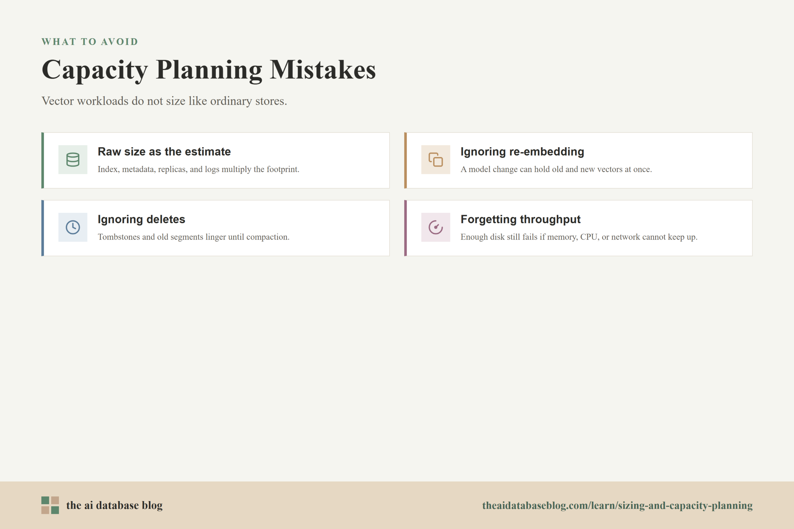
Many capacity problems come from treating vector databases like ordinary key-value stores or document stores. The record count matters, but vector dimension, index structure, and search behavior matter just as much. A system can look small by document count and still be memory-intensive if each document creates many high-dimensional embeddings.
One common mistake is using raw vector size as the full infrastructure estimate. Raw size is only the starting point. Indexes, metadata, replicas, logs, backups, and rebuild space can multiply the footprint. This is especially important for HNSW-style indexes, where graph structures add memory overhead that grows with the number of vectors and index connectivity settings.
Another mistake is planning for today’s dataset without considering growth and re-embedding. If the team later changes embedding models, stores multiple vector fields, adds multilingual embeddings, or reprocesses historical content, capacity can increase quickly. Re-embedding may temporarily require storing old and new vectors at the same time, which means the transition period can be larger than the final state.
A third mistake is ignoring delete and update behavior. Some systems do not immediately reclaim all space when records are deleted or updated. Tombstones, old segments, or fragmented indexes may remain until compaction or rebuilds occur. Capacity plans should leave enough room for this maintenance work, especially in workloads with frequent updates.
Finally, teams sometimes size storage but forget throughput. A deployment can have enough disk capacity and still perform poorly if memory bandwidth, CPU, network, or storage latency cannot support the query and ingestion workload. Capacity planning should therefore be paired with performance testing that reflects real filters, real metadata, real query concurrency, and realistic top-k settings.
These mistakes are avoidable when the sizing process is explicit. The key is to treat each assumption as something that can be measured, not as a fixed truth. That mindset also makes it easier to answer the common questions teams ask when they start planning production vector search.
FAQs
1. How do I estimate the raw size of vectors?
Multiply the number of vectors by the number of dimensions and then by the bytes used for each dimension. For float32 vectors, use 4 bytes per dimension. For example, 1 million vectors with 768 dimensions stored as float32 require about 3.07 GB for the raw vectors before index overhead, metadata, replicas, and operational storage.
2. How much headroom should I add for a vector index?
The right amount depends on the index type, parameters, database implementation, and workload. For early planning with HNSW-style indexes, many teams use a rough overhead range of about 1.3x to 2x the raw vector size, then validate it with the actual system. Additional operational headroom should also be reserved for ingestion, compaction, and rebuilds.
3. Do replicas multiply memory and storage requirements?
Yes, replicas usually multiply the footprint because each copy needs its own data and index structures. If one complete copy requires 400 GB and the deployment keeps three total copies, the replicated footprint is roughly 1.2 TB before backups and temporary overhead. Some architectures share certain storage layers, but the capacity plan should be explicit about what is shared and what is duplicated.
4. Does vector dimension matter more than vector count?
Both matter because they multiply each other. Vector count determines how many objects the system stores, while dimension determines how large each vector is. Doubling either one roughly doubles the raw vector footprint if the data type stays the same. This is why chunking strategy and embedding model choice are both capacity planning decisions.
5. Can quantization reduce capacity needs?
Quantization can reduce memory and storage by representing vectors with fewer bytes per dimension. It can be useful for large datasets, but it should be tested carefully because compression may affect recall, ranking quality, or the need for re-ranking with full-precision vectors. The best choice depends on the accuracy requirements and latency goals of the application.
6. When should I revisit my capacity plan?
Revisit the plan whenever vector count, embedding dimension, metadata size, index settings, replica count, query traffic, or retention policy changes. It is also wise to revisit the estimate after a prototype load test, before a large ingestion run, and before changing embedding models. Capacity planning should become a recurring operational habit rather than a one-time launch task.
Takeaway
Sizing an AI database is easiest when it starts with the raw vector calculation and then adds the real-world layers that production systems need: metadata, index overhead, operational headroom, growth, and replicas. This guidance is most useful for engineers, architects, and technical teams planning vector search, retrieval-augmented generation, semantic search, or recommendation workloads. A practical capacity plan helps teams avoid both underprovisioned systems that struggle under load and oversized deployments that spend too much before the workload requires it.