Benchmarking a vector database means measuring how well it returns the right nearest neighbors under realistic load, not just how fast it can answer easy queries. A fair benchmark defines the workload first, builds exact ground truth with a flat search baseline, then compares approximate search configurations by plotting Recall@K against throughput and tail latency. The goal is to find the best operating point for your application: enough retrieval quality, enough queries per second, and predictable p99 latency under conditions that resemble production.
This guide explains how to design a fair vector database benchmark, why a flat index is commonly used for ground truth, how to measure Recall@K against QPS and p99 latency, and how to avoid synthetic benchmark traps that make systems look better than they will behave in real AI applications. By the end, you should understand how to evaluate vector search performance as a practical tradeoff rather than a single headline number.
What a Vector Database Benchmark Should Actually Measure
A vector database benchmark should answer a practical question: can this system serve the retrieval workload your application needs at the quality and speed your users expect? For an AI application, that usually means the database must find semantically relevant objects, return them quickly, handle concurrent requests, support filters or metadata constraints when needed, and stay predictable as the collection grows or changes.
The most common mistake is treating vector database benchmarking as a raw speed test. Approximate nearest neighbor indexes are designed to trade perfect accuracy for speed. A system can appear extremely fast if it searches less deeply, returns lower-quality neighbors, ignores filters, or avoids returning full objects. That number may be technically true, but it does not tell you whether the retrieval layer is good enough for search, recommendations, RAG, agent memory, or personalization.
A useful benchmark usually includes several kinds of measurement:
- Retrieval quality: How many of the true nearest neighbors are returned at a chosen result size, usually measured as Recall@K.
- Throughput: How many queries per second the system can sustain at a given recall target and latency target.
- Latency: How long individual requests take, especially p95 and p99 latency under concurrent load.
- Indexing behavior: How long it takes to ingest vectors, build or update indexes, and recover from changes.
- Operational realism: Whether the test includes metadata filters, object retrieval, realistic query distributions, and production-like hardware.
Once those measurements are separated, the benchmark becomes much easier to interpret. You are no longer asking which database is fastest in the abstract. You are asking which configuration gives your workload the best balance of recall, throughput, latency, cost, and operational simplicity.
That framing leads to the first major design decision: the benchmark must be fair before it is fast. Without a fair setup, the results may reward shortcuts that your production system cannot actually use.
Designing a Fair Benchmark
A fair vector database benchmark starts with the workload, not the database. Before choosing index parameters or running load tests, define what your application is trying to retrieve, what kinds of queries it receives, how many results it needs, which filters are common, and what latency target matters to users. A benchmark for an internal document retrieval system should not look the same as a benchmark for image similarity, fraud detection, or product recommendations.
The dataset should be representative in size, dimensionality, distance metric, metadata shape, and distribution. If your production vectors are 768-dimensional text embeddings with tenant filters and uneven document popularity, testing only one million uniformly random vectors without filters will give you a weak signal. The benchmark may still be useful as a smoke test, but it will not predict production behavior with enough confidence.
Use the Same Data Model Across Systems
When comparing multiple systems, keep the logical data model consistent. Store the same vectors, the same IDs, the same metadata fields, and the same payload size. If one system returns only vector IDs while another returns full records, the measurement is not comparing the same work. End-to-end query time should include the steps your application actually depends on, including filtering, candidate search, result assembly, and returning the fields needed by the caller.
This matters because vector search performance is not only about distance calculations. Metadata filtering, payload retrieval, network overhead, authorization boundaries, and query parsing can all become meaningful parts of latency. A benchmark that strips those away may be useful for studying an index algorithm, but it is less useful for choosing an AI database architecture.
Control Hardware and Runtime Conditions
Hardware differences can dominate benchmark results. CPU count, memory bandwidth, disk type, cache behavior, network placement, and whether the process is warmed up all affect QPS and latency. For a fair comparison, each database should run with equivalent resources, clear memory limits, comparable client placement, and enough warm-up queries to avoid measuring startup effects instead of steady-state behavior.
Concurrency also needs to match reality. A single-threaded benchmark can show the minimum latency of a system, but most production AI applications serve many users or workers at once. Run tests at multiple concurrency levels and record where latency starts to rise sharply. That inflection point is often more useful than the highest QPS number, because it shows where the system begins to saturate.
Tune Each System Transparently
Approximate indexes have tuning parameters that control the search-quality tradeoff. HNSW-based systems, for example, commonly expose parameters that influence graph construction quality and query-time search depth. IVF-style indexes expose choices such as cluster count and how many partitions to probe. A fair benchmark should tune each system to several operating points rather than freezing every database at a default setting.
The right output is not one row that says one database won. A stronger benchmark shows a curve: at 90 percent recall, what QPS and p99 latency are possible; at 95 percent recall, how much throughput drops; at 99 percent recall, whether latency is still acceptable. This makes the tradeoff visible and prevents a low-recall configuration from looking better than it really is.
With the workload and test conditions defined, the next question is how to know whether returned results are correct. That is where exact search and ground truth come in.
Using a Flat Index for Ground Truth
Recall measurement requires a reference answer. In vector search, that reference is usually produced by exact nearest neighbor search over the same dataset and distance metric. A flat index is commonly used for this purpose because it performs a brute-force comparison between the query vector and the database vectors rather than relying on an approximate index structure. It is slower, but it gives the benchmark a trustworthy answer set.
The process is straightforward. For each benchmark query, run an exact top-K search against the full dataset or a representative subset large enough for the test. Store the resulting neighbor IDs as ground truth. Then run the same query against the vector database configuration being tested and compare the returned IDs with the ground truth IDs.
Why Exact Ground Truth Matters
Approximate nearest neighbor search can miss true neighbors by design. That is acceptable when the speed gain is worth it, but it must be measured. Without exact ground truth, you may only know that the database returned plausible results, not that it returned the nearest available results under the selected metric.
Ground truth also prevents misleading comparisons between index configurations. If one configuration searches deeper and another searches shallower, both may return results that look semantically reasonable. Recall@K shows how much quality each configuration preserved relative to exact search. This lets you compare speed and accuracy on the same scale.
Practical Ground Truth Guidelines
Exact search can be expensive at large scale, so teams often compute ground truth offline. If the full dataset is too large for brute-force comparison on every query, use a representative sample for early experiments and compute full ground truth for the final benchmark queries. Make sure the exact search uses the same vector normalization and distance metric as the database configuration under test. Cosine similarity, dot product, and Euclidean distance can produce different rankings if the vectors are not prepared consistently.
It is also important to save the query set and ground truth results. A repeatable benchmark should be able to rerun the same queries across different versions, index settings, and hardware profiles. Otherwise, performance changes may reflect a new sample of queries rather than a real improvement or regression.
Once exact ground truth exists, Recall@K becomes the main quality metric. But recall by itself is not enough; it only becomes useful when interpreted alongside throughput and tail latency.
Measuring Recall@K
Recall@K measures how many of the true top-K neighbors appear in the top-K results returned by the approximate search system. If the exact top 10 contains 10 specific IDs and the vector database returns 8 of those IDs in its top 10, Recall@10 for that query is 0.8. Average Recall@K is then computed across the benchmark query set.
The value of K should match the application. A RAG system that retrieves 10 chunks for reranking may care about Recall@10. A recommendation system that fills a larger candidate pool may care about Recall@100. A duplicate detection system may care more about whether the single nearest neighbor is correct. Choosing K arbitrarily can distort the results because indexes may behave differently at small and large result sizes.
Do Not Trust Average Recall Alone
Average recall is useful, but it can hide hard-query failures. A system may have strong average Recall@10 while performing poorly on certain query types, sparse regions, dense clusters, filtered queries, or out-of-distribution inputs. In a RAG application, those failures may show up as missing the one document needed to answer a user question, even when the aggregate benchmark looks healthy.
For a more realistic quality picture, report recall distribution as well as the average. Useful additions include median recall, low-percentile recall, the share of queries above a target recall threshold, and recall grouped by query category. This helps reveal whether the system is consistently good or merely good on easy queries.
Measure Filtered and Unfiltered Recall Separately
Metadata filtering changes vector search behavior. Some systems filter before vector search, some search first and filter afterward, and some use specialized filtered-search strategies. These choices affect both speed and recall. If your application uses tenant filters, language filters, document-type filters, timestamps, access rules, or category constraints, filtered recall should be part of the benchmark.
Filtered recall should use ground truth that respects the same filter. For example, if the query asks for the nearest documents where the tenant ID equals a particular value, the exact baseline should search only vectors that satisfy that tenant condition. Comparing filtered approximate results against unfiltered ground truth will produce confusing and unfair scores.
Recall tells you whether the search results are good enough. The next step is to measure how much load the system can handle while preserving that quality.
Measuring QPS Without Losing the Meaning of the Number
Queries per second, or QPS, measures throughput. In vector database benchmarking, QPS is only meaningful when it is tied to a recall target, result size, latency target, dataset size, and hardware profile. Saying a system reached 5,000 QPS does not mean much unless you also know whether that was at Recall@10 of 0.90 or 0.99, whether it returned IDs or full records, and whether p99 latency stayed within the application requirement.
A good QPS benchmark runs at multiple concurrency levels. Start with low concurrency to measure baseline latency. Increase concurrency gradually until throughput plateaus or tail latency becomes unacceptable. This shows both the maximum throughput and the practical throughput you can actually use before users experience slow responses.
Report QPS at a Quality Target
The clearest way to report vector search throughput is to bind it to a quality target. For example, instead of saying the system handled a certain number of queries per second, report QPS at Recall@10 greater than or equal to 0.95 and p99 latency below a defined threshold. This prevents a configuration that sacrifices too much quality from appearing superior.
When comparing index settings, create a table or chart where each row is a configuration and each column includes Recall@K, QPS, p50 latency, p95 latency, p99 latency, memory use, and indexing time. The best choice is usually not the highest-QPS row. It is the row that satisfies the application requirement with the most headroom.
Separate Client Limits From Server Limits
Load generators can become bottlenecks. If the client cannot create enough concurrent requests, serialize responses efficiently, or keep network connections healthy, the benchmark may measure the client instead of the database. Use a load generator with enough CPU and network capacity, run it close enough to avoid accidental wide-area network noise, and monitor both client and server resource utilization.
Also be careful with batching. Batch queries can improve throughput, but they may not match user-facing traffic. If your application sends single interactive queries, benchmark single-query latency and throughput. If your application runs offline batch retrieval, batch performance may be relevant. Mixing the two can make results look better while answering the wrong question.
Throughput shows how much work the system can process. Latency shows what the user or downstream service experiences while that work is happening.
Measuring p99 Latency
Latency percentiles are critical because averages hide slow requests. p99 latency means that 99 percent of measured requests completed at or below that time, while the slowest 1 percent took longer. In user-facing AI systems, that slow tail can dominate perceived reliability. A search system with excellent average latency but unstable p99 latency may cause timeouts, delayed responses, and inconsistent application behavior.
Measure latency from the perspective that matters to the application. If the application calls the database over the network and needs the returned objects, the benchmark should measure end-to-end request latency rather than only internal index lookup time. Internal timings can be useful for debugging, but they should not replace the user-visible measurement.
Watch Tail Latency Under Saturation
p99 latency often stays flat at low concurrency and then rises quickly once the system approaches saturation. That rise can be caused by CPU contention, memory pressure, disk reads, garbage collection, lock contention, network queues, or filter execution paths. This is why QPS and p99 should be plotted together instead of reported separately.
A practical benchmark should identify the highest sustained QPS that keeps p99 latency under the target. If your service-level target is p99 below 100 milliseconds, the useful throughput number is the throughput before p99 crosses that threshold, not the maximum QPS achieved after the system is already overloaded.
Use Warm-Up, Long Enough Runs, and Stable Percentiles
Short benchmark runs can produce noisy percentiles. Run enough queries to make p99 meaningful, especially when testing high concurrency. Warm up the database before measuring so caches, connections, and query execution paths are active. Then run the benchmark long enough to observe steady-state behavior rather than a short burst.
It is also useful to repeat benchmark runs. If results vary widely between runs, investigate before trusting the numbers. Variance can reveal resource contention, background compaction, noisy neighbors, cache sensitivity, or client bottlenecks.
At this point, a benchmark can produce useful curves. The final challenge is making sure those curves represent the real workload rather than an artificial dataset that flatters the index.
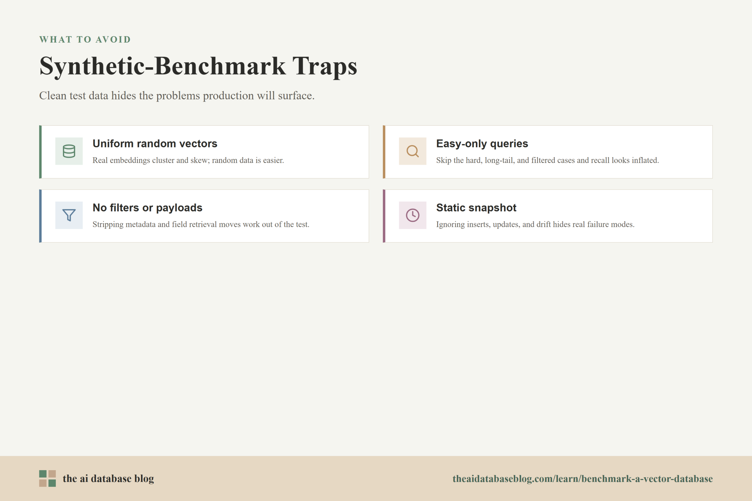
Avoiding Synthetic-Benchmark Traps
Synthetic benchmarks are useful for controlled experiments, but they can mislead when treated as production predictions. Random vectors, uniformly distributed queries, fixed result sizes, and clean metadata can remove the very problems that make vector databases hard to operate. Real data often has clusters, duplicates, changing distributions, uneven popularity, mixed modalities, noisy embeddings, and filters that interact with search quality.
The trap is not using synthetic data at all. The trap is using synthetic data as if it captures production behavior. A benchmark can look excellent on uniformly random vectors because the nearest-neighbor problem is easier or differently shaped than it will be in a real embedding space. Text embeddings, image embeddings, and recommendation embeddings each have their own structure, and that structure affects recall, latency, and memory use.
Use Real Queries Whenever Possible
The query set is as important as the indexed data. Production queries are rarely uniform. Some are repeated often, some are long-tail, some are ambiguous, some target dense topics, and some include filters that shrink the candidate set. If privacy or availability prevents using real queries directly, create a representative query set from anonymized, sampled, or carefully generated examples that preserve the distribution of the workload.
Include hard queries deliberately. For RAG, this may mean queries whose answer depends on a specific document chunk. For recommendations, it may mean cold-start or sparse-profile cases. For semantic search, it may mean short keyword-like queries, long natural-language queries, and queries with exact identifiers. A benchmark that only tests easy queries will overstate production reliability.
Include Metadata Filters and Payload Retrieval
Many AI database workloads are not pure vector searches. They combine vector similarity with filters such as tenant, permissions, language, recency, category, region, or content type. Filtering can change both the candidate set and the index access pattern. If filters are part of the application, benchmark them as first-class scenarios rather than optional extras.
Payload retrieval matters too. Returning only IDs is faster than returning text chunks, metadata, and scores. If the application needs those fields immediately, include them in the measured query path. Otherwise, the benchmark may shift work out of the measurement while still leaving that work for production.
Test Growth, Updates, and Data Drift
A static benchmark does not reveal what happens as vectors are inserted, updated, deleted, or reindexed. Many AI systems continuously ingest documents, refresh embeddings, or remove outdated content. Benchmarking should include indexing throughput, query performance during ingestion, recall after updates, and the operational cost of rebuilding or compacting indexes.
Data drift is another issue. As models change or new content enters the system, vector distributions can shift. A benchmark built only on an old snapshot may miss future failure modes. Periodic benchmarking with fresh samples helps keep the retrieval layer aligned with the application it supports.
Avoiding these traps does not make benchmarking complicated for its own sake. It makes the benchmark honest. The final step is turning the measurements into a repeatable evaluation workflow.
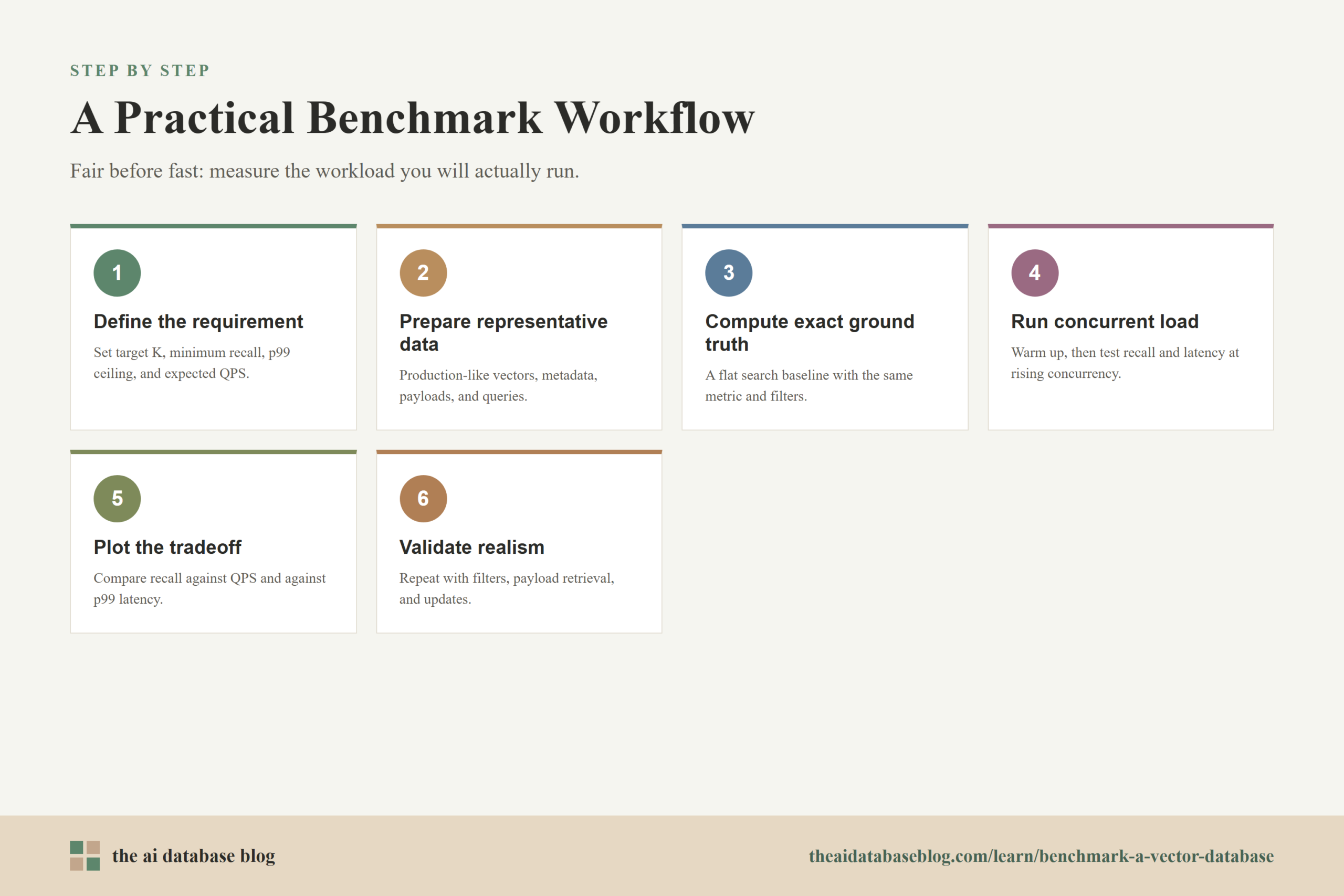
A Practical Benchmark Workflow
A repeatable benchmark should be simple enough to rerun and detailed enough to explain the results. The workflow below is a practical starting point for teams evaluating vector database performance for AI search, RAG, recommendation, or agent memory workloads. It can be scaled up or down depending on the size of the dataset and the risk of the decision.
- Define the application requirement. Decide the target K, minimum Recall@K, maximum p99 latency, expected QPS, filter patterns, and dataset size.
- Prepare representative data. Use production-like vectors, metadata, payload sizes, and query distributions whenever possible.
- Compute exact ground truth. Use a flat exact-search baseline with the same distance metric and filters used in the test.
- Choose configurations to test. Select index parameters that produce different recall and speed points instead of testing only defaults.
- Warm up the system. Run enough queries before measurement to stabilize caches, connections, and execution paths.
- Run concurrent load tests. Measure Recall@K, QPS, p50, p95, p99, error rate, CPU, memory, and disk behavior at multiple concurrency levels.
- Plot the tradeoff curve. Compare configurations by Recall@K versus QPS and Recall@K versus p99 latency.
- Validate production realism. Repeat the test with filters, payload retrieval, updates, and hard query segments.
The most useful result is a decision boundary. For example, you may find that one configuration reaches Recall@10 of 0.96 at the target QPS with p99 below 80 milliseconds, while a higher-recall configuration pushes p99 above the service target. That tells you where to start and what tradeoff you are making.
After the workflow is in place, the benchmark becomes more than a one-time comparison. It becomes a regression test for retrieval quality and performance as data, embeddings, infrastructure, and application requirements change.
How to Interpret Benchmark Results
Interpreting a vector database benchmark means looking for the configuration that satisfies the application, not the configuration that wins every metric. Higher recall is usually better, but it may cost more memory, longer indexing time, lower QPS, or higher p99 latency. Higher QPS is useful, but not if it comes from a search setting that misses too many important neighbors. Lower latency is attractive, but not if the results are too shallow for the downstream task.
Look for stable operating points with headroom. If the system barely meets the p99 target in a quiet benchmark, it may fail during traffic spikes, ingestion bursts, or less favorable query mixes. If recall is strong on average but weak for a known hard segment, the application may still fail in ways users notice. A benchmark should help you find both the average case and the edge cases that need attention.
A good report should include enough context for another person to reproduce or challenge the result. Record dataset size, vector dimensions, distance metric, hardware, memory limits, index settings, query count, concurrency levels, warm-up process, filter patterns, payload size, client location, and software versions. Without that context, benchmark numbers are hard to compare and easy to misuse.
The final interpretation should be written in plain language. For example: this configuration is recommended because it meets Recall@10 of 0.95, sustains the expected traffic with p99 latency below the target, supports the required filters, and leaves enough CPU and memory headroom for normal growth. That kind of conclusion is much more useful than a leaderboard-style ranking.
FAQs
1. What is the most important metric in a vector database benchmark?
There is no single most important metric for every workload. Recall@K, QPS, and p99 latency need to be evaluated together because vector search is a tradeoff between quality and speed. For most production AI applications, the most useful metric is sustained QPS at a required Recall@K and p99 latency target.
2. Why use a flat index for ground truth?
A flat index performs exact nearest neighbor search by comparing the query against the dataset without relying on an approximate search structure. It is slower, but it provides a reliable answer set for measuring how many true neighbors the approximate vector index returned.
3. What does Recall@K mean?
Recall@K measures the fraction of true top-K nearest neighbors that appear in the top-K results returned by the database. If exact search says the true top 10 contains 10 IDs and the database returns 9 of them, Recall@10 for that query is 0.9.
4. Should a benchmark measure average latency or p99 latency?
Both can be useful, but p99 latency is usually more important for production reliability. Average latency can hide slow requests, while p99 latency shows the response time that 99 percent of requests meet or beat. Tail latency is especially important for user-facing search and RAG systems.
5. Are synthetic datasets bad for vector database benchmarking?
Synthetic datasets are not inherently bad. They are useful for controlled experiments and early comparisons. The problem is relying on them as a substitute for production-like data. Real embedding spaces often contain clusters, skew, duplicates, filters, and hard queries that synthetic data may not represent.
6. How often should teams rerun vector database benchmarks?
Teams should rerun benchmarks whenever they change embedding models, index parameters, hardware, database versions, data volume, or major query patterns. For active AI systems, periodic benchmarking is useful because retrieval performance can shift as the dataset grows and the workload changes.
Takeaway
Benchmarking a vector database well means measuring the retrieval system your application will actually use: representative data, exact ground truth, Recall@K, sustained QPS, p99 latency, filters, payload retrieval, and update behavior. This guidance is most useful for teams building AI search, RAG, recommendation, personalization, or agent memory systems where retrieval quality and responsiveness both matter. A strong benchmark does not produce a single universal winner; it shows which configuration meets your quality target, handles your expected load, and stays reliable under realistic conditions.