Product quantization is a vector compression technique used in large-scale similarity search. It works by splitting each high-dimensional vector into smaller subspaces, learning a separate codebook for each subspace, and storing each vector as a compact sequence of codebook IDs instead of full floating-point values. At query time, the system can estimate distances with small lookup tables, which reduces memory use and speeds up search, but it also introduces approximation error that can lower recall if the compression is too aggressive.
This guide explains product quantization from the inside out. It covers why vector databases use it, how subspace splitting works, how codebooks are trained, how compact codes represent vectors, how lookup-table distance computation avoids expensive full-vector comparisons, and how to reason about the compression-versus-recall tradeoff when designing retrieval systems.
Why Product Quantization Matters in Vector Search
Modern AI applications often store millions or billions of embeddings. These embeddings are usually dense vectors made of floating-point numbers, and each vector can have hundreds or thousands of dimensions. A single 768-dimensional vector stored as 32-bit floats uses about 3 KB of memory. That may sound small, but at 100 million vectors it becomes hundreds of gigabytes before accounting for index overhead, metadata, caching, replication, and serving infrastructure.
Product quantization, often shortened to PQ, addresses this memory problem by replacing full-precision vectors with compressed codes. Instead of storing every coordinate as a float, the database stores a small set of integers that point to learned representative patterns. The original vector is no longer stored exactly in the compressed index. It is approximated by a combination of learned centroids, which makes PQ a lossy compression method.
The value of PQ is that it lets a retrieval system keep far more vectors in memory, scan more candidates per query, or reduce infrastructure cost. In many approximate nearest neighbor systems, memory is not just a storage concern; it affects latency because vectors and index structures need to be fetched, compared, and ranked quickly. Smaller representations can improve cache behavior and make large candidate scans more practical.
The cost is that compressed vectors are not perfect copies of the originals. The system is comparing the query against an approximation, so some nearest neighbors may be ranked slightly lower, and some less relevant vectors may move up. Understanding PQ means understanding how it creates that approximation and how much error a particular configuration is likely to introduce.
To see why PQ is more powerful than simply rounding each vector value, it helps to start with the first design choice: the vector is not compressed all at once. It is divided into smaller pieces, and each piece gets its own learned representation.
Splitting Vectors Into Subspaces
Product quantization begins by dividing each vector into multiple fixed-size subvectors. If a vector has 768 dimensions and the system uses 32 subspaces, each subspace contains 24 dimensions. The first subspace might contain dimensions 1 through 24, the second might contain dimensions 25 through 48, and so on until the whole vector has been partitioned.
Each subspace is then treated as its own smaller vector space. This is the key idea behind PQ. Clustering a full 768-dimensional space directly would require a very large codebook to represent the data well. By splitting the vector into lower-dimensional chunks, the system can learn smaller codebooks that are easier to train, store, and search.
The word “product” refers to the way these independent subspace choices combine. If each subspace has 256 possible centroids and there are 32 subspaces, the number of possible reconstructed full vectors is enormous, even though the system only stores 32 small codebooks. A compressed vector is assembled by choosing one centroid from each subspace and concatenating those centroids into an approximate full vector.
This structure gives PQ much of its compression power. Instead of trying to learn one giant list of full-vector prototypes, it learns several smaller lists of subvector prototypes. The combined representation can express many possible vector shapes while keeping the stored code for each individual vector very small.
A Simple Subspace Example
Imagine an 8-dimensional vector split into 4 subspaces of 2 dimensions each. The original vector might look like this:
[0.12, 0.88, 0.44, 0.31, 0.75, 0.18, 0.52, 0.67]
After splitting, the system treats it as four subvectors:
[0.12, 0.88][0.44, 0.31][0.75, 0.18][0.52, 0.67]
Each subvector will be matched to a centroid in its own subspace codebook. The compressed representation does not need to store the two original float values for each subvector. It only needs to store which centroid was closest in that subspace.
Once vectors have been split this way, the next question is where those centroids come from. They are not arbitrary buckets. They are learned from training data so that the compressed representation reflects the actual distribution of vectors in the index.
Learning Codebooks
A codebook is a collection of representative centroids for one subspace. Product quantization learns one codebook per subspace, usually by clustering training subvectors with a method such as k-means. The goal is to choose centroids that represent common patterns in that part of the vector, so that most subvectors can be replaced by a nearby centroid with limited distortion.
If PQ uses 32 subspaces and 8 bits per subspace, each subspace has 256 centroids because 8 bits can represent 256 possible values. During training, the system gathers examples of the first subvector from many training vectors and clusters them into 256 groups. It then repeats the process for the second subvector, the third subvector, and every remaining subspace.
After training, each codebook contains centroids that are specific to its subspace. The centroid for subspace 1 is not used for subspace 2, because the dimensions and data distribution may be different. This matters because embeddings often have uneven structure: some dimensions or groups of dimensions may vary more than others, and some parts of the vector may carry more useful retrieval signal.
The quality of the codebooks strongly affects retrieval quality. If the training sample is too small, outdated, or unrepresentative, the centroids may not match production vectors well. In that case, encoding introduces more error, and recall can fall even if the code size looks reasonable on paper. For AI database workloads, training data should usually reflect the same embedding model, content domain, and data distribution that the index will serve.
What the Codebook Learns
A codebook does not learn concepts in the human sense. It learns geometric representatives. If many subvectors occupy similar positions in a subspace, a centroid can represent that region. When a new vector is encoded, each of its subvectors is assigned to the nearest centroid in the matching codebook.
This nearest-centroid assignment is what creates compression. The system replaces a small floating-point subvector with a small integer ID. The ID says, in effect, “use centroid 173 from codebook 12 for this part of the vector.” Repeating that across all subspaces gives a compact code for the whole vector.
Training explains how PQ creates reusable building blocks. Encoding explains how those building blocks are used to store each database vector, which is where the memory savings become concrete.
Compact Codes: How PQ Stores Vectors
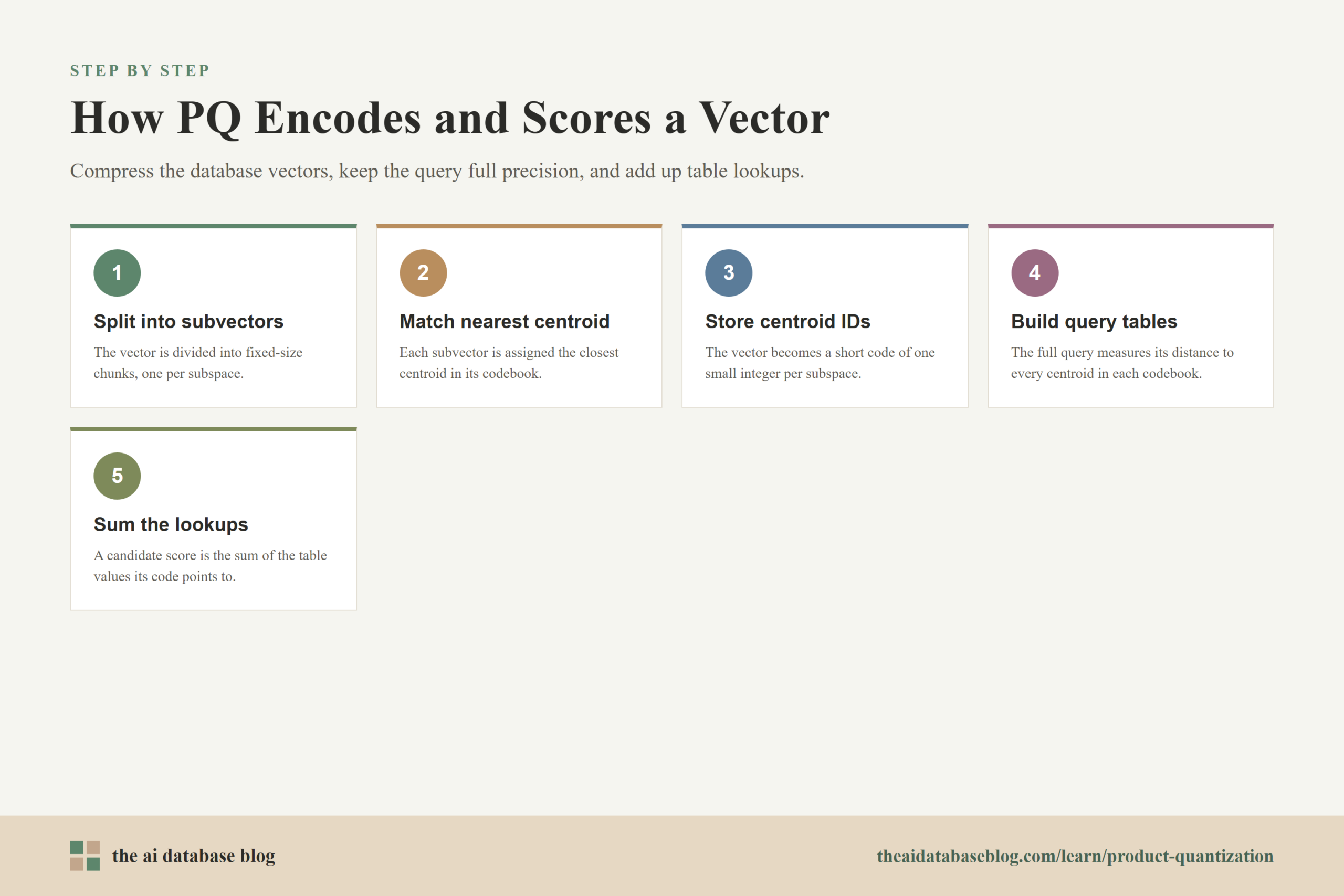
Once the codebooks are trained, each vector can be encoded. The encoder splits the vector into the same subspaces used during training, finds the closest centroid for each subvector, and stores the centroid ID. The result is a compact code made of one small value per subspace.
For example, a vector split into 8 subspaces might be represented as:
[14, 201, 87, 3, 155, 42, 19, 230]
Each number points to a centroid in the corresponding subspace codebook. If each number is stored in one byte, this code uses only 8 bytes. By contrast, a 128-dimensional vector stored as 32-bit floats uses 512 bytes. That is a 64-to-1 reduction for the vector payload itself. Real index memory depends on surrounding data structures, but the vector representation becomes dramatically smaller.
The compressed code can also be decoded into an approximate vector by concatenating the selected centroids. Decoding is useful for explanation, reconstruction, or certain index operations, but search systems often avoid fully reconstructing every candidate. Reconstructing millions of vectors would give up much of the efficiency that PQ was meant to provide.
Instead, PQ search usually works directly with the compact codes. The query remains full precision, while the database vectors are compressed. The search engine estimates the distance between the query and each compressed vector by using precomputed lookup tables.
Code Size and Bit Depth
The code size depends on two main settings: the number of subspaces and the number of bits per subspace. More subspaces usually means more code entries per vector. More bits per subspace means each entry can choose from a larger codebook. Both can improve approximation quality, but both increase memory or computation in some way.
A common configuration is 8 bits per subspace, which gives 256 centroids per codebook and makes each subspace ID fit cleanly in one byte. Smaller bit depths, such as 4 bits, can produce even smaller codes and may improve some low-level CPU behaviors, but they also reduce the number of centroids available to represent each subspace. Larger bit depths increase representational flexibility, but they create larger lookup tables and may reduce some of the practical speed benefit.
At this point, PQ has turned full vectors into short codes. The next important step is understanding how a database can compare a full query vector to those codes without reconstructing every stored vector one by one.
Lookup-Table Distance Computation
The most common search pattern for PQ is asymmetric distance computation, often called ADC. It is asymmetric because the query vector stays in full precision while the database vectors are represented by compressed codes. This usually gives better accuracy than compressing both the query and the database vector before comparing them.
When a query arrives, the system splits the query into the same subspaces used by the product quantizer. For each query subvector, it computes the distance to every centroid in the corresponding codebook. The result is a set of small lookup tables. If there are 32 subspaces and 256 centroids per subspace, the query creates 32 tables with 256 distance values each.
After those tables are built, estimating the distance to a compressed database vector becomes simple. The system reads the code for that database vector, looks up the precomputed distance for each selected centroid, and adds the values together. Instead of calculating a full distance across all original dimensions, it performs a series of table lookups and additions.
For a code such as [14, 201, 87, 3], the approximate distance is computed by adding:
- the distance between query subvector 1 and centroid 14 in codebook 1,
- the distance between query subvector 2 and centroid 201 in codebook 2,
- the distance between query subvector 3 and centroid 87 in codebook 3,
- the distance between query subvector 4 and centroid 3 in codebook 4.
The sum is not the exact distance to the original vector. It is the distance to the PQ approximation of that vector. In practice, this is often good enough to identify a strong candidate set, especially when followed by reranking against full-precision vectors or by using a less aggressive PQ configuration.
Why Lookup Tables Are Fast
Lookup-table computation is fast because the expensive query-to-centroid distances are calculated once per query, not once per database vector. After that, each candidate comparison is reduced to small memory reads and additions. This is especially useful when a search system needs to scan many compressed candidates inside an inverted file list, a graph neighborhood, or another approximate nearest neighbor structure.
The performance benefit is not automatic in every environment. Table size, CPU cache behavior, SIMD optimizations, memory bandwidth, and index design all matter. Still, the basic principle is durable: PQ makes distance estimation cheaper by moving most arithmetic into a small per-query table and representing database vectors as compact codebook choices.
Now that the mechanics are clear, the practical question becomes how much compression is acceptable. The answer depends on recall requirements, data scale, latency goals, and whether the system can rerank candidates using more accurate representations.
The Compression-Versus-Recall Tradeoff
Product quantization trades exactness for efficiency. Stronger compression reduces memory use and can improve scan speed, but it also increases quantization error. Quantization error is the gap between the original vector and the approximation reconstructed from selected centroids. The larger that gap becomes, the more likely the search system is to misorder nearby candidates.
Recall measures whether the search system returns the true nearest or most relevant neighbors according to a reference method. In a compressed index, recall can drop because PQ changes the distances being compared. If two candidate vectors are very close in the original space, small approximation errors can be enough to swap their order. If a relevant vector is moved too far away by compression, it may never reach the final result set.
This does not mean PQ is inaccurate by default. Many large-scale retrieval systems use it effectively because the memory savings allow them to search more data, keep more candidates in RAM, or allocate resources to reranking. The tradeoff is not simply “compression bad, full precision good.” The real question is whether the compression error is acceptable for the application and whether the system design compensates for it.
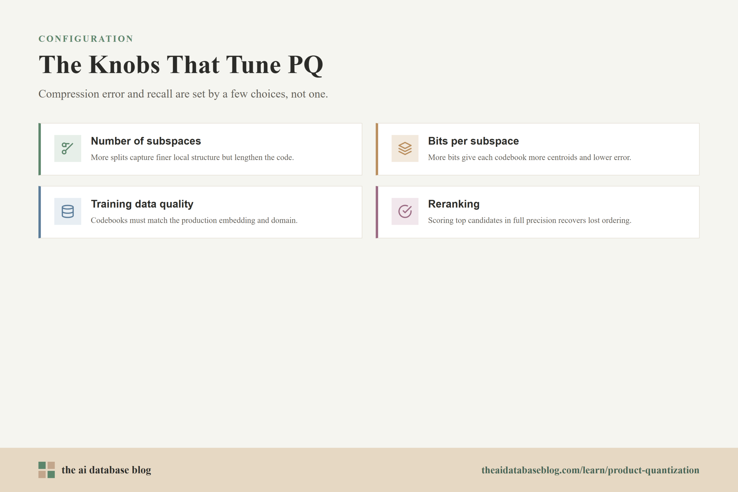
The main tuning knobs are the number of subspaces, the number of bits per subspace, the quality of training data, and the use of reranking. Increasing the number of bits per subspace gives each codebook more centroids, which can reduce error. Increasing the number of subspaces can represent more local structure, but it also changes subvector size and code length. Better training data helps codebooks match the vectors being encoded. Reranking can recover accuracy by taking a larger approximate candidate set and scoring the top candidates with full-precision vectors or a stronger model.
How to Think About the Tradeoff in Practice
A practical PQ configuration should be chosen through evaluation, not guesswork. Start with the target use case: semantic search for internal documents may tolerate some approximate ordering if the top results are still useful, while retrieval for a high-stakes decision workflow may require higher recall and more conservative compression. The more the application depends on exact nearest-neighbor ordering, the more careful the PQ settings need to be.
Teams usually evaluate PQ by comparing compressed search results against a full-precision or higher-accuracy baseline. Useful measurements include recall at a chosen result count, latency, memory footprint, throughput, and downstream answer quality for retrieval-augmented generation. For RAG systems, it is not enough to measure vector recall alone. The final question is whether compression causes the retriever to miss context that the generator needs.
A good rule of thumb is to use PQ when memory pressure is high enough that exact storage or full-precision scanning becomes impractical, and then spend part of the savings on broader candidate retrieval or reranking. PQ is often most effective as part of a larger retrieval architecture rather than as a standalone quality shortcut.
The same tradeoff appears differently depending on how PQ is combined with the rest of the index. That is why it helps to understand where PQ sits inside an AI database or vector search system.
Where PQ Fits in an AI Database
In an AI database, product quantization is usually one part of the retrieval stack. The system may first use metadata filters to limit the search space, then use an approximate nearest neighbor index to identify candidates, then use PQ to store or scan those candidates efficiently, and finally rerank a smaller set with more accurate scoring. PQ is a compression and distance-estimation technique, not a complete retrieval strategy by itself.
PQ is commonly paired with coarse partitioning methods. For example, an inverted index can assign vectors to broad clusters, search only the most relevant clusters for a query, and use PQ codes to score compressed vectors inside those clusters. This combination reduces both the number of candidates searched and the cost of scoring each candidate. Graph-based systems can also use quantization to reduce memory pressure while navigating or scoring candidates.
For RAG workloads, PQ can be useful when the corpus is large, embeddings are high dimensional, and the application needs low-latency retrieval. However, RAG systems also care about result usefulness, not just nearest-neighbor metrics. Compression that slightly lowers vector recall may or may not affect generated answers, depending on whether the missed documents contain unique information and whether reranking or hybrid search can recover the right context.
Metadata filtering also changes the PQ decision. If filters narrow the candidate set heavily, the system may not need aggressive compression because fewer vectors are compared. If filters are broad or the corpus is very large, PQ can make the difference between searching enough candidates and being forced into a smaller, less reliable candidate set.
When PQ Is a Good Fit
Product quantization is a strong fit when the dataset is large, memory is a limiting factor, and approximate retrieval is acceptable. It is especially useful when the system can evaluate quality with real queries and tune the configuration against recall, latency, and cost targets. PQ is also attractive when the compressed index enables a larger candidate scan than would be possible with full-precision vectors.
PQ is less attractive when the dataset is small enough to store and search in full precision, when exact ordering is required, or when the embedding distribution changes frequently enough that codebooks become stale. It can also be risky when there is no evaluation set, because teams may compress aggressively without noticing the retrieval quality they have lost.
Choosing PQ well means treating it as an engineering lever. It can unlock scale, but it should be tuned with the same care as chunking, embedding selection, hybrid search, filtering, and reranking.
Common PQ Configuration Choices
The most important PQ choices are easy to describe but subtle to optimize. The number of subspaces determines how many parts the vector is split into. The number of bits per subspace determines how many centroids each codebook can contain. Together, these settings define the compressed code size and influence the amount of approximation error.
For a vector with dimensionality d, using m subspaces creates subvectors of size d / m, assuming the dimensionality divides cleanly. If the system uses b bits per subspace, each subspace can represent 2^b centroid choices. The approximate code size is m * b bits per vector, plus any index overhead and stored metadata.
As a concrete example, a 768-dimensional float vector uses 3,072 bytes at 32-bit precision. With 64 PQ subspaces and 8 bits per subspace, the compressed code is 64 bytes. That is a large reduction in vector storage, but it is not automatically the best setting. The right choice depends on how much recall the application needs and how well the codebooks fit the data.
Some systems also use variations such as optimized product quantization, residual quantization, scalar quantization, binary quantization, or reranking with stored original vectors. These techniques solve related problems, but the core PQ idea remains the same: divide the vector space, learn subspace codebooks, store centroid IDs, and estimate distances from compressed representations.
Questions to Ask Before Using PQ
- How large is the vector corpus? PQ becomes more valuable as the memory cost of full-precision vectors grows.
- What recall target does the application need? A recommendation interface, support search system, and compliance workflow may have very different tolerance for missed neighbors.
- Will the system rerank candidates? Reranking can reduce the user-visible impact of approximate first-stage retrieval.
- Is the training data representative? Codebooks trained on the wrong distribution can add avoidable error.
- How often do embeddings change? A new embedding model can require retraining codebooks and re-encoding vectors.
These questions make PQ easier to reason about as a production choice. The algorithm is mathematically compact, but its value depends on how it behaves under real query traffic, real data distributions, and real quality constraints.
FAQs
1. What is product quantization in simple terms?
Product quantization is a way to shrink large vectors by replacing parts of each vector with IDs that point to learned representative patterns. Instead of storing every floating-point value, the system stores a short code. During search, that code is used to estimate similarity or distance without fully reconstructing the original vector.
2. Why does product quantization split vectors into subspaces?
Splitting vectors into subspaces makes the compression problem easier. Learning one codebook for a full high-dimensional vector would require many centroids to represent the data well. By learning separate codebooks for smaller subvectors, PQ can combine many simple choices into a flexible full-vector approximation.
3. What is a codebook in product quantization?
A codebook is a set of centroids learned for one vector subspace. Each centroid represents a common subvector pattern found in the training data. When a vector is encoded, each of its subvectors is assigned to the nearest centroid in the matching codebook, and the centroid ID becomes part of the vector’s compact code.
4. How does lookup-table distance computation work?
For each query, the system computes the distance between each query subvector and every centroid in the corresponding codebook. These distances are stored in small lookup tables. To score a compressed database vector, the system reads the vector’s compact code, looks up the relevant centroid distances, and adds them together.
5. Does product quantization always reduce recall?
Product quantization introduces approximation error, so it can reduce recall if the compressed representation changes nearest-neighbor rankings. However, the effect depends on the code size, codebook quality, data distribution, search strategy, and reranking. In some systems, PQ can support good practical recall by allowing the database to search more candidates within the same memory or latency budget.
6. When should an AI database use product quantization?
An AI database should consider PQ when vector memory is a bottleneck, the corpus is large, and approximate retrieval is acceptable. It is most useful when the team can measure recall and downstream quality, tune compression settings, and use reranking or larger candidate pools to balance efficiency with relevance.
Takeaway
Product quantization helps AI databases store and search large vector collections by splitting embeddings into subspaces, learning codebooks for those subspaces, storing compact centroid IDs, and estimating query distances through lookup tables. It is most useful for engineers and technical teams building retrieval systems where memory, latency, and scale matter, especially in large semantic search or RAG applications. The main lesson is that PQ is not just a compression trick: it is a relevance tradeoff that should be tuned and evaluated against real recall targets, real query behavior, and the quality requirements of the application.