Pre-filtering, post-filtering, and in-graph filtering are three ways to combine vector similarity search with metadata constraints. Pre-filtering applies the constraint before or during candidate selection, which usually protects recall but can increase latency when the filter is restrictive. Post-filtering runs vector search first and removes non-matching results afterward, which is simple and often fast, but it can miss valid matches unless the system over-retrieves. In-graph filtering integrates the filter into approximate nearest neighbor traversal, especially in graph indexes such as HNSW, so the system can search toward relevant vector neighborhoods while remaining aware of which objects satisfy the filter.
This guide explains how each filtering strategy works, why each one affects recall and latency differently, how over-retrieval helps post-filtering, and why modern systems increasingly combine structured filters with graph traversal instead of treating filtering as a separate step. By the end, you should understand how to reason about filtered vector search behavior in AI databases and retrieval systems.
Why Filtered Vector Search Matters
Vector search is useful because it retrieves objects by semantic similarity rather than exact keyword overlap. A query such as “refund policy for enterprise customers” can find passages that discuss cancellation terms, billing disputes, and account-level support even when those exact words are not present. In real applications, though, semantic similarity alone is rarely enough. The system often needs to restrict results by tenant, language, document type, access permission, publication date, geography, product category, or some other structured condition.
That combination creates the filtered vector search problem. The database must find the nearest vectors among only the objects that satisfy a filter. In a retrieval-augmented generation system, for example, the application may need the top 10 semantically relevant passages where customer_id = 42, source = policy, and language = English. The filter is not just a display preference. It defines which results are allowed to participate in the answer.
The hard part is that approximate nearest neighbor indexes are built to avoid scanning every vector. Graph-based indexes such as HNSW move through a connected structure of nearby vectors and stop when they have found enough promising candidates. Filters can interrupt that process. If many nearby vectors are not eligible, the system has to decide whether to skip them, traverse through them, search a separate subset, widen the search, or accept fewer results.
Once filtering becomes part of the retrieval path, the placement of the filter matters. The next sections explain the three main strategies: pre-filtering, post-filtering, and in-graph filtering.
Pre-Filtering
Pre-filtering applies the structured condition before the final vector results are chosen. In its simplest form, the system first identifies all objects that match the filter, then performs vector search only over that eligible set. In more integrated systems, the filter may be converted into an allow list that is passed into the vector index, so the index can consider filter eligibility while searching. The core idea is the same: the top results should be selected from the filtered population, not from the full unfiltered dataset.
Mechanics
A pre-filtered query usually starts with a metadata lookup. The system uses a scalar index, inverted index, bitmap, column index, or similar structure to find object identifiers that satisfy the filter. For a condition such as department = legal and status = published, the filter engine can produce a set of eligible IDs. The vector search then uses that set as the population from which nearest neighbors should be returned.
There are two common implementation patterns. The first is exact search over the filtered subset. If the filter returns a small number of objects, the system may compute vector distance for every eligible object and return the best matches. This can be very accurate and surprisingly efficient when the subset is small. The second pattern is approximate search with an allow list. The graph or vector index still performs approximate traversal, but only candidates that satisfy the filter can be accepted as final results.
Recall Implications
Pre-filtering usually has strong recall semantics because the system is asking the right question: “What are the nearest neighbors inside the filtered set?” If there are at least k eligible matches and the search is exact, it can return the correct top k for that filtered population. If the search is approximate, recall still depends on index configuration, traversal breadth, and stopping rules, but the system is at least trying to retrieve from the eligible set rather than hoping eligible objects appear in an unfiltered candidate list.
The recall challenge appears when the filtered subset is difficult for an approximate graph to navigate. In HNSW, the graph is organized around vector proximity across the whole dataset. A filter can create a sparse or disconnected slice of that graph. If only a small percentage of nodes match the filter, the search may have to traverse many non-matching nodes before it finds enough eligible candidates. Some systems handle this by switching to exact search when the filtered subset is small enough.
Latency Implications
Pre-filtering can be fast when the filter is selective and the filtered subset is small. In that case, the metadata index quickly narrows the candidate population, and exact vector comparison over that subset may be cheaper than a broad approximate search over the full index. This is especially true when the filter is something like a tenant ID, document collection, or narrow time range.
Latency can rise when the filter is selective but the vector index still needs to traverse a large graph to find enough eligible nodes. The cost is no longer only the cost of the vector search; it also includes filter evaluation, allow-list checks, and potentially broader traversal. For filters that match a large share of the dataset, pre-filtering may add overhead without narrowing the search much. This is why production systems often use query planners or thresholds to decide whether to use exact filtered search, approximate filtered search, or another strategy.
Pre-filtering gives the system clean retrieval semantics, but it is not always the lowest-latency option. That tension is why post-filtering remains common, especially in systems that need a simple way to combine existing vector search with structured constraints.
Post-Filtering
Post-filtering applies the structured condition after vector search has already produced candidates. The vector index first retrieves the nearest results from the full dataset without regard to the filter. The system then removes results that do not satisfy the filter and returns the remaining items. This approach is straightforward because it does not require the vector index to understand metadata constraints during traversal.
Mechanics
A post-filtered query usually has two stages. First, the approximate nearest neighbor index returns a candidate list such as the top 10, top 100, or top 1,000 nearest vectors from the full dataset. Second, the filter engine checks each candidate against the structured condition. If the query asks for 10 results but only 4 of the retrieved candidates match the filter, the system may return 4 results unless it performs additional retrieval.
This makes post-filtering easy to implement but sensitive to candidate size. The vector search is optimized for semantic closeness across all objects, not for eligibility. If the closest objects are mostly outside the filter, they crowd out valid filtered objects that are slightly farther away. Those valid objects may never reach the candidate list, so the filter never gets a chance to accept them.
Recall Implications
Post-filtering can reduce recall because the filter is applied after the approximate search has already truncated the candidate pool. The system may miss relevant filtered results even when those results exist in the database. This is especially likely when the filter is highly selective, when the desired k is small, or when the eligible objects are not concentrated near the query in vector space.
For example, imagine a dataset with 1 million support articles and a filter that restricts results to one customer’s private documents. If the system retrieves the top 20 vectors globally, most or all of those candidates may come from other customers. After filtering, the result set may be empty, even though the customer has useful matching documents farther down the global ranking. The problem is not that the documents are irrelevant. The problem is that they were never retrieved before the filter was applied.
Latency Implications
Post-filtering often has predictable vector-search latency because the index does the same kind of unfiltered traversal it would normally do. The filter check happens afterward and is usually cheap for a small candidate list. This can make post-filtering attractive for broad filters where most top vector results are likely to pass the condition.
The tradeoff is that achieving acceptable recall may require retrieving many more candidates than the application ultimately returns. That extra retrieval increases distance computations, memory access, network transfer, reranking work, and downstream processing. Post-filtering may look fast when the candidate list is small, but that speed can come from silently accepting recall loss.
Over-Retrieval for Post-Filtering
Over-retrieval is the main mitigation for post-filtering. Instead of retrieving exactly the requested k, the system retrieves a larger candidate set and then filters it down. If the application needs 10 final results, the system might retrieve 100, 500, or 1,000 unfiltered candidates before applying the filter. The hope is that enough eligible objects appear somewhere in the larger candidate pool.
A simple way to think about over-retrieval is to estimate filter selectivity. If a filter matches roughly 10 percent of the dataset and the application needs 10 final results, retrieving 100 candidates may produce about 10 eligible candidates on average. If the filter matches only 1 percent, the system may need around 1,000 candidates on average. Real retrieval is less tidy than this estimate because filter membership and vector similarity are often correlated or anti-correlated, but selectivity gives a useful starting point.
requested results = 10
estimated filter match rate = 10 percent
rough candidate count = 10 / 0.10 = 100

requested results = 10
estimated filter match rate = 1 percent
rough candidate count = 10 / 0.01 = 1,000
Over-retrieval improves the odds of finding enough filtered results, but it does not guarantee correct recall. If eligible objects are far below the global top candidates, even a large candidate pool may miss them. It also increases latency and resource use. For restrictive filters, post-filtering can become either inaccurate with a small candidate list or expensive with a large one.
Post-filtering is useful when filters are broad and implementation simplicity matters. But as filters become more selective, retrieval systems need a way to preserve recall without blindly expanding the candidate pool. That is where in-graph filtering becomes important.
In-Graph Filtering
In-graph filtering integrates filter awareness into approximate nearest neighbor traversal. Instead of treating the metadata condition as a separate pre-step or post-step, the search algorithm uses the filter while moving through the vector graph. This is especially relevant for HNSW-style indexes, where search starts from one or more entry points and follows neighbor links toward vectors that appear closer to the query.
Mechanics
In a graph-based vector index, each object is connected to nearby objects. A normal unfiltered search evaluates candidate nodes, follows promising edges, and maintains a set of nearest candidates. With in-graph filtering, the traversal still uses graph structure, but it also checks whether nodes satisfy the filter. The system may allow non-matching nodes to help traversal continue through the graph while only admitting matching nodes into the final result set.
Modern implementations go beyond a simple “skip non-matching nodes” rule. If the system skips too aggressively, it can break graph navigation because non-matching nodes may be necessary bridges to reach matching neighborhoods. More advanced approaches use filter-aware entry points, allow lists, multi-hop exploration, selective distance calculations, or predicate-aware subgraph traversal. The goal is to search efficiently inside the filtered population without losing the navigability of the original graph.
Recall Implications
In-graph filtering is designed to improve recall compared with naive post-filtering because eligible nodes are considered throughout the search process. The algorithm is not limited to whichever eligible objects happen to appear in the unfiltered top candidates. Instead, it can keep exploring until it has found enough matching candidates or until its stopping conditions indicate that additional traversal is unlikely to improve the result.
Recall still depends on implementation details. A filtered traversal must balance two needs: using non-matching nodes as pathways through the graph and prioritizing matching nodes as candidate answers. If the filter is extremely restrictive, even an in-graph strategy may approach exhaustive behavior or switch to exact search. If the filter is moderately selective, in-graph filtering can often preserve better recall than post-filtering without the full cost of brute-force search.
Latency Implications
Latency in in-graph filtering depends on filter selectivity, vector-filter correlation, and traversal design. If the filter aligns well with the vector neighborhood, the search may find matching candidates quickly. For example, a query about German tax documents with a language filter for German may naturally move through areas of the graph where many candidates pass the filter. In that case, filter-aware traversal can be efficient.
If the filter is poorly correlated with vector similarity, latency can rise. The graph may lead the search into semantically relevant regions where many objects fail the filter. Advanced traversal strategies try to address this by seeding filter-matching entry points, widening exploration, evaluating neighborhoods in larger hops, or choosing exact search when the eligible set is small. The practical goal is not to make every filtered query equally fast, but to avoid the worst behavior of both naive pre-filtering and naive post-filtering.
In-graph filtering is best understood as a family of integrated retrieval strategies rather than a single algorithm. That distinction matters because modern systems often combine filtering modes dynamically.

How Modern Systems Integrate Filters Into Traversal
Modern vector systems increasingly treat filtered search as a query planning problem. Instead of using one fixed strategy for every query, they estimate how restrictive the filter is, how many results are requested, how large the dataset is, and how expensive the index traversal is likely to be. Based on those signals, the system may choose exact search over a filtered subset, approximate traversal with an allow list, post-filtering with over-retrieval, or a filter-aware graph traversal strategy.
Allow Lists and Metadata Indexes
One common integration pattern is to build an allow list from a metadata index and pass that list into vector search. The graph traversal can still move through the HNSW structure, but the result set is constrained to eligible IDs. This keeps structured filtering close to the vector retrieval path and avoids the most obvious post-filtering failure mode, where valid filtered results are never considered.
Filter-Aware HNSW Traversal
Another pattern is to adapt graph traversal itself. Instead of evaluating all nodes the same way, the algorithm uses filter information to decide which candidates should receive distance calculations, which neighborhoods should be explored, and how to reach filtered regions faster. Some systems use strategies inspired by predicate subgraph traversal, where the search tries to emulate movement through the subgraph of eligible objects while still relying on the original graph for connectivity.
Fallbacks to Exact Search
For very restrictive filters, exact search over the filtered subset can be the most efficient and reliable path. If a filter narrows a million-object dataset down to a few hundred eligible records, computing exact vector distances for those few hundred records may beat approximate graph traversal. This is why some systems use a threshold: below a certain filtered subset size, they switch to flat or exhaustive search.
Planner-Based Strategy Selection
The most practical systems combine these techniques. A query planner can use selectivity estimates, index statistics, shard layout, and query parameters to decide how to execute the filtered search. This is important because the same filter strategy can behave very differently across workloads. A category filter that matches 40 percent of records is a different problem from a tenant filter that matches 0.1 percent. A filter that is correlated with the query vector is different from one that excludes most nearby semantic neighbors.
This integrated view makes the comparison more useful. The question is not simply which filtering strategy is best. The better question is which strategy fits the filter selectivity, recall requirement, latency budget, and structure of the data.
Comparing Recall and Latency Tradeoffs
Each filtering strategy makes a different compromise between retrieval quality and execution cost. Pre-filtering starts with the eligible population, so it often has the cleanest recall semantics. Post-filtering starts with the nearest unfiltered vectors, so it often has simpler execution but weaker recall under selective filters. In-graph filtering tries to keep the speed benefits of graph traversal while making the traversal aware of filter constraints.
| Strategy | How it works | Recall behavior | Latency behavior | Best fit |
|---|---|---|---|---|
| Pre-filtering | Builds an eligible set before selecting vector results. | Usually strong because results are selected from the filtered population. | Fast for small subsets, but graph traversal can become expensive for restrictive filters. | High-recall queries, tenant filters, permission filters, narrow structured constraints. |
| Post-filtering | Runs vector search first, then removes candidates that fail the filter. | Can miss valid results, especially with selective filters or small candidate pools. | Predictable for small candidate lists, but over-retrieval can increase cost. | Broad filters, simple implementations, low-risk retrieval where occasional misses are acceptable. |
| In-graph filtering | Uses filter awareness during graph traversal and candidate acceptance. | Often better than post-filtering because eligible candidates are searched for during traversal. | Can be efficient for moderate filters, but still depends on selectivity and correlation. | Filtered ANN workloads that need both relevance quality and lower latency. |
The most important practical lesson is that recall and latency should be measured together. A post-filtered query may appear fast because it retrieves too few eligible results. A pre-filtered query may appear slower because it is doing the work required to find the correct filtered top results. An in-graph approach may reduce that cost, but it still needs careful evaluation under realistic filters.
How to Choose a Filtering Strategy
The right strategy depends on how selective the filter is and how costly a missed result would be. For RAG systems, access control and tenant isolation filters should usually be treated as hard constraints where recall and correctness matter. For exploratory search, recommendation, or broad category browsing, a small amount of recall loss may be acceptable if latency is more important. The retrieval design should reflect the risk of missing a valid result.
Use pre-filtering or exact filtered search when the eligible set is small, when filters represent permissions, or when returning fewer than k results would create a bad user experience. Use post-filtering only when filters are broad enough that the unfiltered top candidates are likely to include sufficient eligible results, or when the system can safely over-retrieve. Use in-graph filtering when the workload needs approximate search at scale but cannot tolerate the recall problems of naive post-filtering.
It also helps to track filter selectivity in production. Log how many objects match common filters, how many candidates are retrieved before filtering, how many survive filtering, and how often the final result count is below the requested k. These measurements reveal whether a strategy is actually working or simply hiding failures behind a fast response time.
Once a team understands those measurements, filtered vector search becomes easier to tune. The next step is to apply a few practical rules that keep retrieval quality visible.
Practical Rules for AI Database Workloads
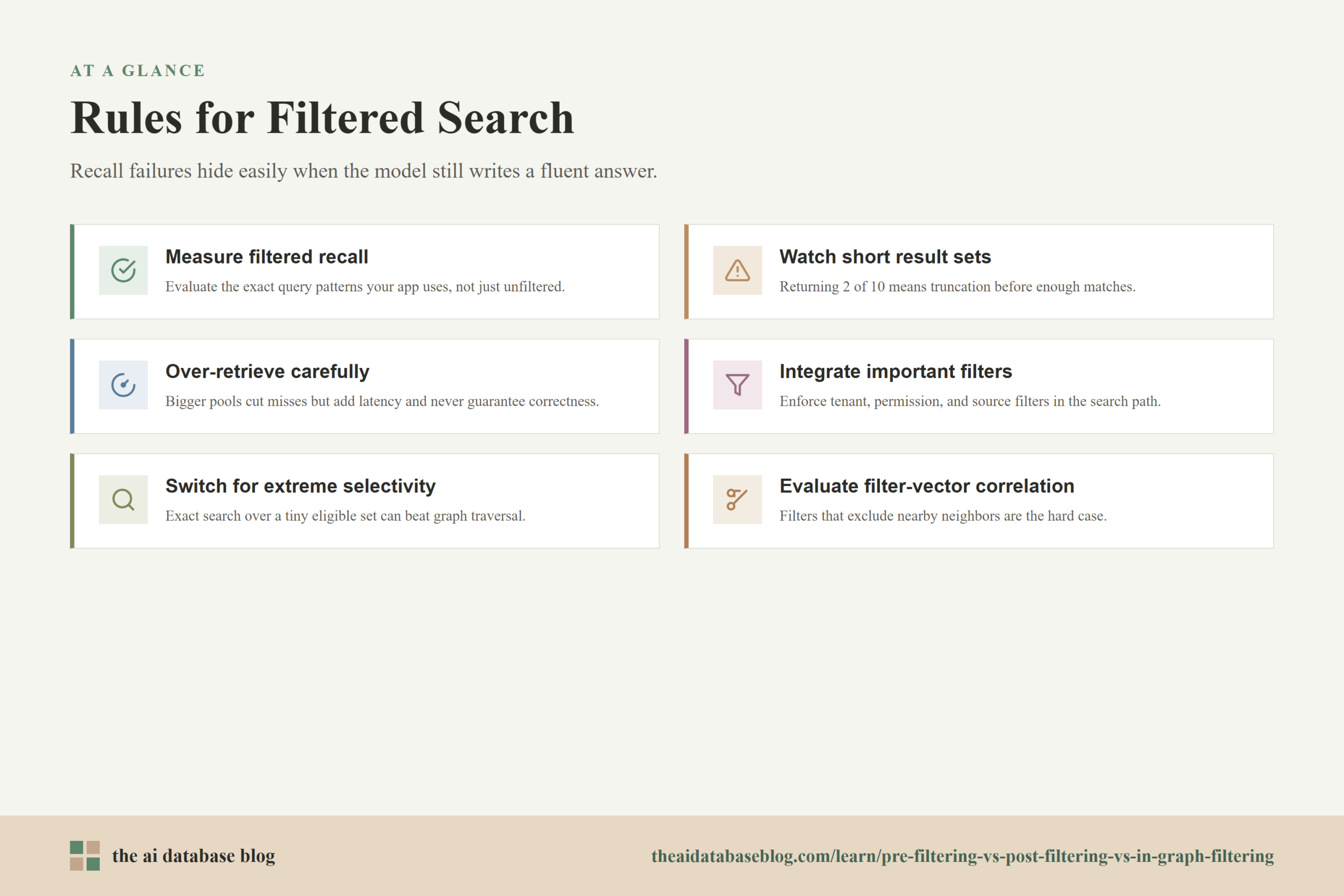
Filtered vector search should be designed around the application’s tolerance for missing relevant results. In AI database workloads, the retrieval layer often feeds a generated answer, an agent decision, or a user-facing knowledge result. That makes recall failures harder to notice because the application may still produce a fluent answer from incomplete evidence.
- Measure filtered recall, not just unfiltered recall. A vector index can perform well on ordinary nearest neighbor benchmarks while failing under metadata constraints. Evaluate the exact query patterns your application uses.
- Watch for empty or short result sets. If a query asks for 10 results and post-filtering regularly returns 2, the system is probably truncating before it has found enough eligible candidates.
- Use over-retrieval carefully. Larger candidate pools can reduce post-filtering misses, but they also increase latency and do not guarantee correctness under very selective filters.
- Prefer integrated filtering for important constraints. Permission, tenant, compliance, and source-of-truth filters should be enforced in the retrieval path, not treated as a cosmetic cleanup step after retrieval.
- Switch strategies for extreme selectivity. When the filtered subset is very small, exact search over that subset can be more reliable and sometimes faster than approximate graph traversal.
- Evaluate filter-vector correlation. Filters that align with vector neighborhoods are easier to handle than filters that exclude most nearby semantic candidates. This affects both recall and latency.
These rules are not tied to one vendor or one index type. They are general principles for reasoning about vector search systems that combine embeddings with structured metadata.
FAQs
1. What is the main difference between pre-filtering and post-filtering?
Pre-filtering applies the metadata condition before the final vector results are selected, so the search is focused on eligible objects. Post-filtering applies the condition after vector search has already returned candidates from the full dataset, so eligible objects can be missed if they were not in the original candidate list.
2. Why can post-filtering return fewer than the requested number of results?
Post-filtering can return fewer than the requested number because the vector index retrieves unfiltered candidates first. If many of those candidates fail the filter, the remaining result set may be smaller than k, even when more matching objects exist elsewhere in the database.
3. Does over-retrieval solve post-filtering recall problems?
Over-retrieval helps but does not fully solve the problem. Retrieving more unfiltered candidates increases the chance that enough filtered results appear in the candidate pool, but it can still miss valid matches when the filter is highly selective or poorly correlated with vector similarity. It also increases latency and resource use.
4. Why can pre-filtering be slower for restrictive filters?
Pre-filtering can be slower when the vector index has to traverse a large graph to find enough eligible nodes. A restrictive filter may exclude many nearby vectors, forcing the search to expand farther through the graph. Some systems respond by switching to exact search over the filtered subset when that subset is small.
5. What does in-graph filtering mean?
In-graph filtering means the filter is used during approximate nearest neighbor graph traversal. The system remains aware of metadata eligibility while moving through the graph, accepting only matching objects as final candidates while still using graph structure to find semantically relevant regions.
6. Which filtering strategy is best for RAG?
For RAG, the best strategy depends on the filter. Hard constraints such as tenant, permission, language, or source filters usually need pre-filtering, exact filtered search, or in-graph filtering because recall and correctness matter. Post-filtering may be acceptable for broad, low-risk filters when enough over-retrieval is used and result quality is measured.
Takeaway
Pre-filtering, post-filtering, and in-graph filtering are different ways of answering the same question: how should an AI database find the nearest vectors that also satisfy structured constraints? Pre-filtering gives the cleanest filtered retrieval semantics, post-filtering is simple but often needs over-retrieval to avoid missed results, and in-graph filtering reflects where modern systems are heading by integrating filters into traversal itself. This guidance is most useful for teams building RAG, semantic search, recommendation, or agent memory systems where metadata constraints affect both correctness and performance, especially when a query must retrieve relevant content from a restricted tenant, permission group, document source, or time window.