k-nearest neighbours, often shortened to k-NN, is the retrieval operation that finds the k stored items most similar to a query. In AI databases, those items are usually vectors created from text, images, audio, code, or other data, and similarity is measured with a distance or similarity function such as cosine similarity, dot product, or Euclidean distance. Exact k-NN checks the available vectors directly and returns the true closest results, while approximate k-NN uses an index to return highly likely neighbours much faster at large scale. The value of k controls how many candidates are returned, and many production retrieval systems intentionally retrieve more results than they finally need so a reranker can choose the best few.
This guide explains what happens during a k-NN operation, why exact and approximate nearest-neighbour search behave differently, how to choose k for common AI database applications, and why over-retrieving followed by reranking is often the practical choice for retrieval-augmented generation, semantic search, recommendations, and other AI systems.
What k-Nearest Neighbours Means in an AI Database
In an AI database, k-nearest neighbours is a way to ask, “Which stored objects are closest to this query in meaning or representation?” The database stores vectors, also called embeddings, that place related items near one another in a high-dimensional space. A user question, product description, image, or document chunk can be embedded into the same kind of vector, then compared with the stored vectors to find nearby matches.
The “k” simply means the number of neighbours requested. If k is 5, the system returns the five closest matches it can find according to the configured distance metric and retrieval method. If k is 50, it returns a broader set of nearby candidates. The operation is simple in concept, but the engineering details matter because modern embedding collections can contain millions, billions, or more vectors.
It helps to separate k-NN as a mathematical idea from k-NN as a production database operation. The mathematical idea is to rank all candidate items by closeness to the query. The production operation must do that under constraints such as latency, memory, filters, updates, security rules, and downstream use by a search page, recommender system, or language model.
Once the basic idea is clear, the next natural question is what the database actually does when a query arrives. The operation has a few repeatable steps, and understanding those steps makes it much easier to reason about exact search, approximate search, and the effect of changing k.
The k-NN Operation Step by Step
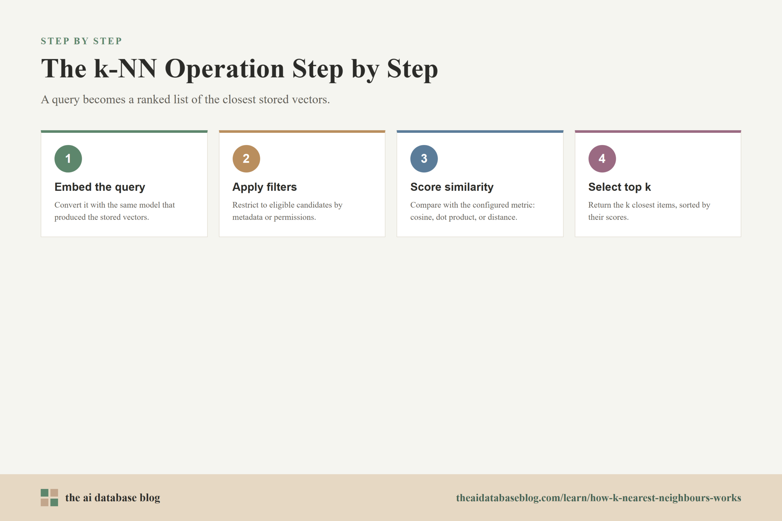
A k-NN query starts with a query object and ends with a ranked list of nearby stored objects. In semantic search, the query object may be a sentence or question. In recommendation, it may be a user profile, a recent interaction, or an item vector. In duplicate detection, it may be a document, image, or record that needs to be compared with existing items.
1. Convert the query into a vector
The query must be represented in the same vector space as the stored data. If the collection contains text embeddings from one embedding model, the query should usually be embedded with the same model or a compatible model. This matters because vector distance is only meaningful when the vectors share the same representation. A query vector from a different embedding space may produce rankings that look numeric but are not semantically reliable.
2. Apply filters when the query requires them
Many AI database queries combine vector similarity with metadata constraints. A support assistant may search only documents from a certain product version. An ecommerce system may search only in-stock products. A compliance workflow may search only records a user is allowed to access. Filtering can happen before, during, or after vector search depending on the database design, but the goal is the same: compare the query with eligible candidates rather than irrelevant or unauthorized data.
3. Compute or estimate similarity
The retrieval system compares the query vector with candidate vectors using a configured metric. Cosine similarity focuses on direction, dot product can reflect direction and vector magnitude, and Euclidean distance measures straight-line distance. The right metric depends on how the embeddings were trained and normalized. In many systems, the embedding model or database configuration determines the expected metric, so changing it casually can harm relevance.
4. Select the top k results
After scoring candidates, the system returns the k closest items. In exact k-NN, these are the true nearest neighbours among the searched candidates. In approximate k-NN, they are the best results found by the index under the chosen speed, memory, and recall settings. The returned list is usually sorted by distance or similarity score, though downstream applications may reorder it later.
This step-by-step view shows why k-NN is more than a single distance calculation. It is a pipeline that depends on the embedding model, eligible candidate set, similarity metric, index strategy, and final result count. The biggest implementation choice is whether to search exactly or approximately, because that decision shapes both accuracy and scale.
Exact k-NN Search
Exact k-NN search returns the true nearest neighbours for the query within the searched set. The straightforward version compares the query vector with every eligible stored vector, computes a distance or similarity score for each one, and keeps the best k. This is sometimes called brute-force search, but that name can be misleading because exact search can still be optimized with batching, hardware acceleration, caching, and efficient top-k selection.
The main advantage of exact k-NN is reliability. If the data set is small enough, the latency acceptable, and the vectors available in a format that can be scanned efficiently, exact search removes one source of retrieval error. This is useful when the application needs the highest possible recall, when evaluation requires ground-truth neighbours, or when the collection is small enough that approximation is unnecessary.
The limitation is cost at scale. Comparing one query vector against every eligible vector becomes expensive as the number of vectors, vector dimensions, and concurrent queries increase. Even when hardware can handle exact search for some workloads, an application may still choose approximate search to reduce latency, memory bandwidth, or infrastructure cost.
Exact search gives a useful baseline: it tells you what the nearest neighbours are if the system spends enough work to find them. Approximate search starts from a different assumption. It asks how much exactness can be traded for speed while still returning results that are good enough for the user or downstream model.
Approximate k-NN Search
Approximate k-NN, often called ANN search, uses an index to avoid comparing the query with every vector in full detail. Instead of exhaustively scoring all candidates, the system narrows the search to promising regions, graph paths, clusters, compressed representations, or other structures that make retrieval faster. The result is usually much lower latency and better scalability, with the tradeoff that the returned top k may miss some true nearest neighbours.
Graph-based indexes
Graph-based ANN indexes connect vectors to nearby vectors and search by navigating through those connections. HNSW, or Hierarchical Navigable Small World, is a widely used example. It builds layered proximity graphs so search can move quickly across broad regions before refining toward closer neighbours. These indexes are popular because they often provide a strong balance between recall and latency when the index can fit in memory.
Partition-based indexes
Partition-based indexes divide the vector space into clusters or lists, then search only the most relevant partitions for a query. Inverted file indexes are a common example. Instead of scanning all vectors, the system identifies a smaller set of likely partitions and compares the query with vectors inside them. Searching more partitions can improve recall, while searching fewer partitions can reduce latency.
Compression-based indexes
Compression-based methods store smaller or lower-precision representations of vectors so comparisons use less memory and compute. Product quantization is a well-known technique in this family. Compression can make very large indexes more practical, but compressed distances are approximate. Many systems therefore use compression for candidate discovery and then refine the best candidates with more accurate vector representations.
Approximate search is not a single algorithm but a family of tradeoffs. The important practical question is not whether ANN is “accurate” in the abstract. It is whether the index settings return enough relevant candidates, quickly enough, for the application. That leads directly to choosing k, because k controls how broad or narrow the returned neighbourhood is.
How to Choose k for Different Applications
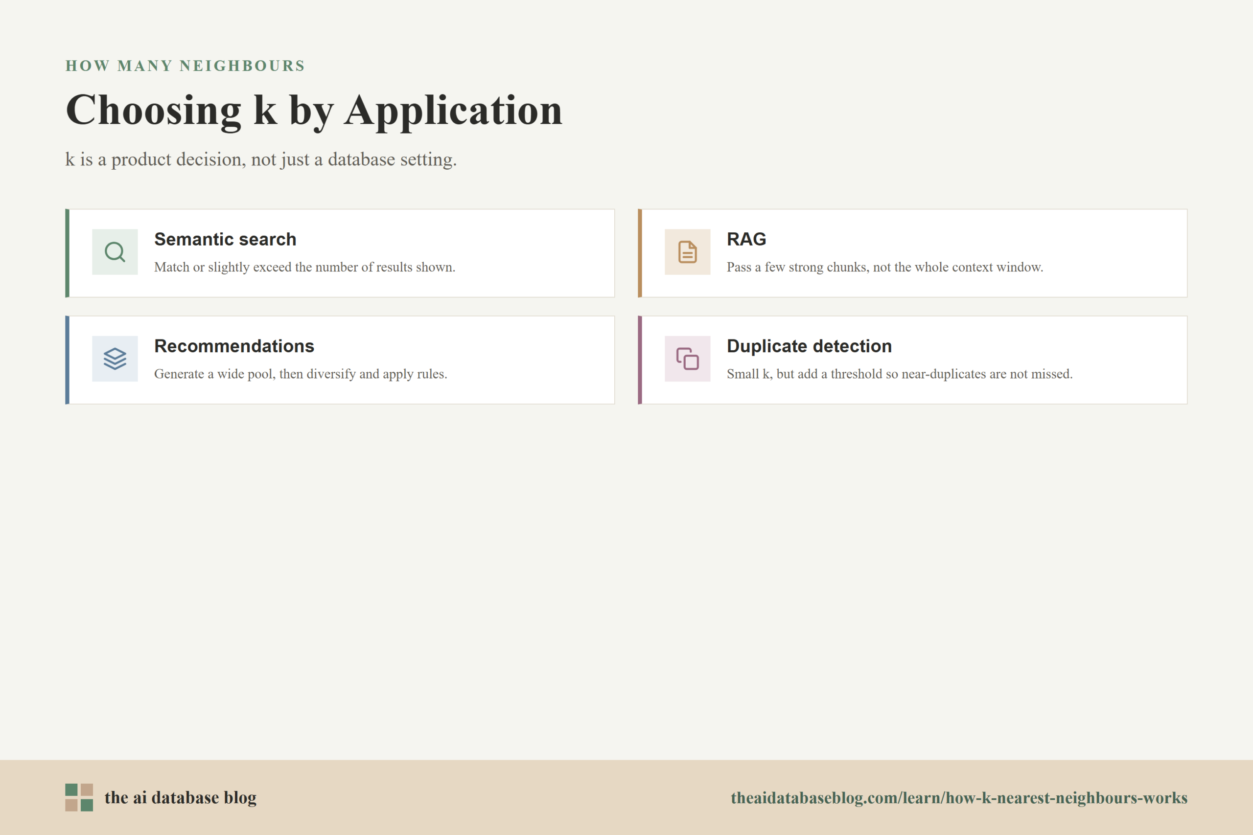
Choosing k is an application decision, not just a database setting. A small k gives a focused result set, which can improve precision and reduce downstream cost. A larger k gives the system more chances to include relevant items, which can improve recall. The best value depends on how many results the user or model will actually use, how noisy the embedding space is, whether reranking is available, and how costly each additional result is.
Semantic search
For a search interface where users see a page of results, k should often match or slightly exceed the number of results displayed. If the page shows 10 results, retrieving 10 to 20 may be reasonable for a simple system. If the system uses reranking, personalization, permissions, or result grouping, it may retrieve 50 or more candidates and then narrow them down. The goal is to avoid missing strong candidates while keeping the visible list precise.
Retrieval-augmented generation
For RAG, k should be chosen around the context that the language model can use effectively, not merely the maximum context window size. Sending too few chunks can cause missing evidence. Sending too many chunks can add distraction, contradictions, or irrelevant details. A common pattern is to retrieve a wider candidate pool, rerank it, and pass only a smaller final set to the model, such as the best 4 to 10 chunks depending on chunk size and task complexity.
Recommendations
Recommendation systems often benefit from a larger candidate pool because the nearest items may later be diversified, filtered, or balanced against business rules and user preferences. The first-stage k may be dozens, hundreds, or more, while the final displayed set may be much smaller. In this setting, k is part of candidate generation rather than the final user-facing ranking.
Duplicate detection and clustering workflows
Duplicate detection may use a small k if the goal is to find the most likely duplicates for manual review or automated matching. However, if false negatives are costly, the system may use a larger k plus a similarity threshold so it does not miss near-duplicates that sit just outside the first few results. Clustering and analysis workflows may also vary k depending on whether they need local neighbourhood structure or broad candidate coverage.
Classification with k-NN
In classical k-NN classification, k controls the number of labelled neighbours that vote on the predicted class. A very small k can be sensitive to noise. A very large k can blur local distinctions by including points from other classes or regions. Although AI database retrieval is often different from supervised k-NN classification, the same intuition applies: k should be large enough to be stable, but not so large that it dilutes the signal.
These examples show that k is a relevance and product-design choice as much as a retrieval parameter. But k also interacts with ranking quality. If the first-stage vector ranking is imperfect, a small k can hide the right answer just below the cutoff. That is why many systems separate candidate retrieval from final ranking.
Over-Retrieving and Then Reranking
Over-retrieving means asking the first-stage retriever for more results than the application will finally use. For example, a RAG system might retrieve the top 50 vector matches, rerank those 50 using a more precise model or scoring method, and send only the best 5 to the language model. This pattern is common because first-stage retrieval is optimized for speed and coverage, while reranking is optimized for precision.
The reason this works is that candidate generation and final ranking solve different problems. The first stage should make sure the right answer is somewhere in the candidate pool. The second stage should decide which candidates are most useful for the exact query. A vector search index may be excellent at finding semantically similar text, but a reranker can often better judge whether a passage directly answers a question, matches a rare term, resolves an entity, or provides the right evidence.
Common reranking signals
Reranking can use several signals. A cross-encoder model can score a query and candidate together, which is often more precise than comparing independently generated embeddings but more expensive per candidate. A system can also recompute exact distances on original full-precision vectors after an approximate or compressed search. Other reranking approaches may combine vector score, keyword score, metadata freshness, authority, access rules, diversity, or application-specific relevance features.
Why not just set k very high?
Simply increasing k is not the same as improving retrieval quality. A larger k may include more relevant candidates, but it also includes more noise. In a search page, that noise can push good results down. In a RAG system, too much irrelevant context can make the generated answer less focused. Over-retrieving works best when it is paired with a second stage that reduces the broad candidate set to a smaller, cleaner final set.
How much should you over-retrieve?
There is no universal multiplier, but the first-stage candidate pool should be large enough to catch relevant items that might not rank perfectly in the initial vector search. For small, clean collections, retrieving 2 to 3 times the final result count may be enough. For noisy, diverse, or high-stakes retrieval, a system may retrieve 5 to 20 times the final count and use evaluation to decide whether the extra candidates improve recall without causing unacceptable latency.
Over-retrieval and reranking make k a two-stage decision. There is the candidate k used by the retriever and the final k used by the application. To choose both well, teams need evaluation metrics that reflect the role each stage plays.
How to Evaluate k-NN Retrieval Quality
Evaluation should measure whether the retrieval system returns useful results, not just whether it runs quickly. For AI database applications, the most important metrics often include recall at k, precision at k, mean reciprocal rank, and nDCG. These metrics answer different questions: did the system include the relevant item, did it keep the top results clean, did it rank the first useful result early, and did it order graded relevance well?
For exact versus approximate search, recall is especially important. ANN recall usually compares approximate results with exact nearest-neighbour results for the same query set. If approximate search consistently captures the true nearest neighbours at the needed k, it may be a good tradeoff. If it misses important results, the system may need different index settings, a larger candidate pool, better filtering, or a reranking stage.
For RAG, retrieval evaluation should also connect to answer quality. A retriever can return semantically related chunks that do not actually contain the answer. That is why teams often evaluate whether the gold evidence appears in the candidate set, whether the reranker moves it into the final context, and whether the generated answer uses it correctly. The right k is the value that improves the whole pipeline, not just the nearest-neighbour score.
Once evaluation is in place, tuning becomes less speculative. Instead of asking whether k should be 5, 10, or 50 in general, you can ask which value improves recall, precision, latency, and downstream quality for your own queries and data.
Practical Guidelines for Using k-NN in AI Databases
Good k-NN retrieval starts with the data and ends with the application. The database can only compare the vectors it has, so embedding quality, chunking strategy, metadata design, and filtering rules all affect the result. Index choice and k settings matter, but they cannot fully compensate for poorly structured data or unclear retrieval goals.
- Use exact search as a baseline when practical, especially during evaluation. It helps reveal whether approximation is causing misses or whether the issue lies in embeddings, chunking, filters, or ranking.
- Use approximate search when scale, latency, or memory make exact search too expensive. Tune index parameters against recall and latency rather than assuming default settings are optimal.
- Choose k based on the number of useful results the application can consume. A user interface, a recommender, and a RAG prompt may need very different final result counts.
- Separate candidate k from final k when using reranking. Retrieve enough candidates to protect recall, then rerank and trim the final set for precision.
- Evaluate with real queries and relevance judgments. Synthetic examples can help during development, but production tuning needs queries that reflect actual user behavior and data distribution.
These guidelines keep k-NN grounded in practical retrieval rather than abstract nearest-neighbour theory. The best systems treat k as one part of a larger design that includes embeddings, filters, indexing, candidate generation, reranking, and measurement.
FAQs
1. What does k mean in k-nearest neighbours?
k is the number of nearest results the system should return. If k is 10, the system returns the 10 closest candidates according to its distance metric and search method. In AI databases, k is often used for vector search over embeddings, where the nearest neighbours are the stored items most similar to the query vector.
2. Is k-NN the same as vector search?
Vector search often uses k-NN, but the two terms are not exactly identical. k-NN describes the operation of finding the k closest items. Vector search is the broader database capability for searching vector embeddings, often with filters, indexes, scoring choices, and sometimes hybrid keyword-and-vector retrieval.
3. When should exact k-NN be used?
Exact k-NN is useful when the data set is small enough to scan efficiently, when the application requires the true nearest neighbours, or when you need a ground-truth baseline for evaluating approximate search. It can also be practical with strong hardware acceleration or narrow filtered candidate sets.
4. Why do vector databases use approximate nearest-neighbour search?
Vector databases use approximate nearest-neighbour search because exact comparison can become too slow or expensive for large, high-dimensional collections. ANN indexes reduce the number of comparisons, make comparisons cheaper, or both. The tradeoff is that the system may miss some true nearest neighbours, so teams tune ANN settings based on recall, latency, memory, and application needs.
5. How do I choose the right k for RAG?
For RAG, choose k based on how much evidence the language model can use effectively. A small final k, such as a handful of well-ranked chunks, is often better than filling the context with loosely related text. Many systems retrieve a larger candidate pool first, rerank it, and pass only the strongest final chunks to the model.
6. What is the difference between over-retrieving and reranking?
Over-retrieving is the act of retrieving more candidates than the application will finally use. Reranking is the second-stage process that reorders those candidates with a more precise signal. They work together: over-retrieval improves the chance that relevant items are in the pool, and reranking improves the chance that the best items appear at the top.
Takeaway
k-nearest neighbours is the core operation behind many AI database retrieval systems: embed the query, compare it with eligible stored vectors, and return the k closest matches. Exact k-NN gives the true nearest neighbours but can be expensive at scale, while approximate k-NN uses indexes such as graph, partition, or compression-based methods to trade some exactness for speed and efficiency. The right k depends on the application, the downstream consumer, and the cost of missing relevant results. For teams building semantic search, RAG, recommendations, or duplicate detection, the most practical pattern is often to retrieve a broad candidate set, rerank it with a stronger signal, and return a smaller final set that balances recall, precision, and latency.