Approximate nearest neighbor indexes trade some search accuracy for speed because they avoid comparing a query vector with every vector in the database. Instead of doing exhaustive search, they use shortcuts such as graph navigation, clustering, compressed representations, candidate pruning, or staged reranking. The main tuning question is how much work the index should do per query: more work usually improves recall, while less work usually lowers latency and increases queries per second.
This guide explains why that trade-off exists, how common ANN parameters control it, and how to read a recall-versus-QPS curve when choosing an operating point. By the end, you should understand why there is no single best ANN setting, how to reason about recall targets, and how to pick a search configuration that fits the real user experience of an AI application.
Why ANN Search Exists
Vector search starts with a simple goal: given a query embedding, find the stored embeddings that are most similar to it. In exact nearest neighbor search, the database compares the query against every candidate vector and returns the closest matches. This can produce the most accurate result set for a given similarity function, but it becomes expensive as the collection grows, especially when vectors are high-dimensional and queries must be served with low latency.
Approximate nearest neighbor search exists because many AI applications do not need a mathematically exhaustive scan for every request. They need relevant results quickly enough to support a product experience such as retrieval-augmented generation, semantic search, recommendations, deduplication, or clustering. ANN indexes reduce the amount of work needed at query time by organizing vectors so the system can inspect a promising subset of candidates instead of the whole dataset.
The word approximate is important. ANN search is not usually trying to return random good-enough results. It is trying to return nearly the same neighbors that exact search would return, but with far less computation. Recall measures how much of the exact result set the ANN result set recovered. Latency measures how long the query took. QPS, or queries per second, measures throughput under load. These three metrics are connected because higher recall usually requires the index to explore more candidates, evaluate more distances, or perform more reranking.
Once you see ANN search as controlled candidate selection, the recall-latency trade-off becomes easier to understand. The next question is why every ANN index has this trade-off, even though different index families use very different data structures.
Why Every ANN Index Trades Accuracy for Speed
Every ANN index trades accuracy for speed because it intentionally avoids some comparisons that exact search would perform. The index may skip distant clusters, stop graph exploration early, search only a subset of partitions, use compressed vector representations, or rerank only a small candidate pool. Each shortcut saves time, memory bandwidth, or CPU and GPU work. The cost is that the true nearest neighbor may be hidden behind a path, partition, or candidate set the query did not inspect.
This is not a flaw in ANN search. It is the design principle that makes ANN search useful. If an index performed all possible comparisons, it would become exact search. The practical value of ANN indexing is that many vectors can be safely ignored for a specific query because the index has learned or constructed enough structure to guide the search toward likely matches.
Graph-Based Indexes
Graph-based indexes, such as HNSW-style indexes, connect vectors to nearby vectors in a navigable graph. At query time, the search starts from an entry point and walks through the graph toward increasingly similar candidates. This can be very fast because the search does not need to inspect every vector. However, the graph walk can miss a better neighbor if it does not explore widely enough or if the graph structure does not provide a good path to that neighbor.
The accuracy-speed trade-off in graph search is mainly controlled by how many candidate paths the search keeps alive. A narrow search finishes quickly but may settle into a local neighborhood that is close but not optimal. A wider search explores more alternatives, improves the chance of finding the same results as exact search, and costs more time per query.
Cluster-Based Indexes
Cluster-based indexes, often described as inverted file or IVF-style indexes, divide the vector space into partitions. At query time, the system identifies the most promising partitions and searches within them. This avoids scanning the full dataset, but it can miss relevant vectors if a true neighbor lives in a partition that was not probed.
The trade-off is controlled by how many partitions the query searches. Probing more partitions increases recall because the query sees a broader candidate pool. Probing fewer partitions improves latency and throughput because the query touches less data. The right setting depends on how cleanly the data clusters, how many results are needed, and how much latency the application can tolerate.
Quantized and Compressed Indexes
Quantized indexes reduce memory use and speed up distance calculations by storing compressed approximations of vectors. This can make large-scale search much more efficient, especially when memory bandwidth is a bottleneck. The trade-off is that compressed vectors may not preserve all fine-grained similarity differences, so the approximate ranking can differ from the exact ranking over full-precision vectors.
Many production systems handle this by using a two-stage process. First, the compressed index quickly retrieves a candidate set. Then the system reranks some candidates using full vectors or more precise scores. A larger reranking set tends to improve recall and ranking quality, but it also adds latency and resource use.
These index families use different mechanics, but they all ask the same operational question: how much search work is enough? That question is answered through tuning parameters.
How ANN Parameters Control Recall and Latency
ANN parameters are the controls that decide how aggressively the index searches. Some parameters affect the index at build time, such as graph density, construction quality, clustering granularity, or compression strength. Other parameters affect the query itself, such as the number of explored candidates, searched partitions, or reranked results. Build-time parameters often shape the maximum quality the index can reach, while query-time parameters decide how much of that potential quality is spent on each request.
The most important practical lesson is that most ANN parameters are not simply good or bad. They move the system along a curve. A setting that is too low may be fast but miss important matches. A setting that is too high may recover more exact neighbors but consume latency budget that the user never notices or cannot afford.
Search Breadth Parameters
Search breadth parameters control how many candidates the index considers during a query. In graph indexes, this is often a candidate list or exploration width. In cluster-based indexes, it is often the number of partitions searched. In compressed or staged systems, it may be the number of candidates passed into reranking.
Increasing search breadth is the most direct way to raise recall. The query explores more of the index, compares against more candidates, and has a better chance of finding the true nearest neighbors. The trade-off is higher latency per query and lower QPS because each request consumes more compute and memory access. Search breadth is often the first parameter to tune because it can usually be changed without rebuilding the index.
Graph Density and Construction Quality
Graph indexes also have build-time parameters that affect how richly connected the graph is and how carefully neighbors are chosen during insertion. A denser or better-constructed graph can improve recall because queries have more useful paths through the data. It can also reduce the amount of query-time exploration needed to reach a recall target.
The trade-off is that denser graphs use more memory and take longer to build or update. They can also increase the cost of each exploration step because there are more connections to evaluate. This means a stronger index structure may improve the recall curve, but it is not free. Teams usually tune graph construction after they understand whether query-time breadth alone can meet their target.
Partition Count and Probe Count
Cluster-based indexes depend on how vectors are assigned to partitions and how many partitions are searched per query. More partitions can make each searched partition smaller, which may improve speed, but it can also make recall sensitive to whether the right partitions are probed. Fewer partitions may reduce routing complexity but can require scanning more vectors within each partition.
The query-time probe count is the main recall-latency control. A low probe count produces high QPS but may miss neighbors outside the closest partitions. A higher probe count improves recall by widening the search area. The best setting is usually found empirically because it depends heavily on the embedding model, data distribution, vector dimensionality, and filtering behavior.
Compression and Reranking Parameters
Compressed indexes add another layer to the trade-off. Stronger compression can reduce memory footprint and improve throughput, but it may lower ranking precision. Reranking can recover quality by rescoring a candidate pool with more accurate representations. The key parameter is how many candidates are reranked before returning the final top results.
A small reranking pool may be fast but unable to recover a missed neighbor. A larger pool improves the chance that the correct candidates survive the approximate first stage, but it adds extra scoring work. For retrieval systems that feed a language model, reranking is often worth testing because a modest increase in retrieval latency can improve answer quality if it reliably brings better context into the prompt.
These parameters are meaningful only when measured against the application goal. A search configuration is not successful because it has the highest possible recall. It is successful when it reaches enough recall within the latency, throughput, memory, and cost limits of the system.
How to Measure Recall, Latency, and QPS
To tune an ANN index responsibly, you need a measurement setup that compares approximate results against a reliable reference. The usual approach is to create a representative query set, run exact search or a trusted high-recall baseline to produce ground truth, and then compare ANN results at different parameter settings. This lets you measure how much quality you gain or lose as you move along the speed curve.
Recall should be measured at the same result depth the application uses. If the application retrieves 10 chunks for a RAG prompt, recall at 10 is more meaningful than recall at 1. If the system displays 20 search results, recall at 20 may matter more. The metric should reflect the actual user or downstream model behavior, not just a convenient benchmark default.
Recall
Recall measures the fraction of exact nearest neighbors that appear in the ANN results. If exact search says the top 10 results should contain a particular set of items, and the ANN result contains 9 of those 10 items, recall at 10 is 90 percent for that query. Averaged across many queries, recall gives a practical view of how often the ANN index recovers the neighbors that exact search would have returned.
Recall is useful because it separates retrieval quality from later ranking, generation, or business logic. However, recall does not always equal user-perceived quality. Some missed neighbors may be near-duplicates of returned items. Some exact nearest neighbors may be less useful than semantically diverse context. For that reason, recall is best used alongside application-level evaluation, especially in RAG systems.
Latency
Latency measures how long a query takes. Average latency is helpful, but tail latency is often more important in user-facing systems. A system with good average latency but poor p95 or p99 latency may feel inconsistent because some users wait much longer than others. ANN tuning should therefore consider both typical and worst-case query behavior.
Latency also changes under load. A query setting that looks fine in a single-threaded benchmark may perform differently when many requests compete for CPU, GPU, memory bandwidth, cache, disk, or network resources. This is why latency should be measured under realistic concurrency rather than only in isolated tests.
QPS
QPS measures how many queries per second the system can serve at an acceptable latency. It is closely related to latency, but it is not identical. A system can sometimes serve individual queries quickly at low load but fail to maintain that latency as throughput increases. Conversely, a setting with slightly higher per-query latency may still be acceptable if it keeps the system stable and predictable under expected traffic.
When reading recall-versus-QPS curves, remember that QPS depends on hardware, dataset size, vector dimension, filtering, batching, concurrency, and implementation details. The curve is most useful for comparing settings under the same test conditions. It should not be treated as a universal benchmark that transfers unchanged across systems.
Once the metrics are clear, the next step is to read the curve itself. This is where ANN tuning becomes a practical product and infrastructure decision rather than a purely algorithmic one.
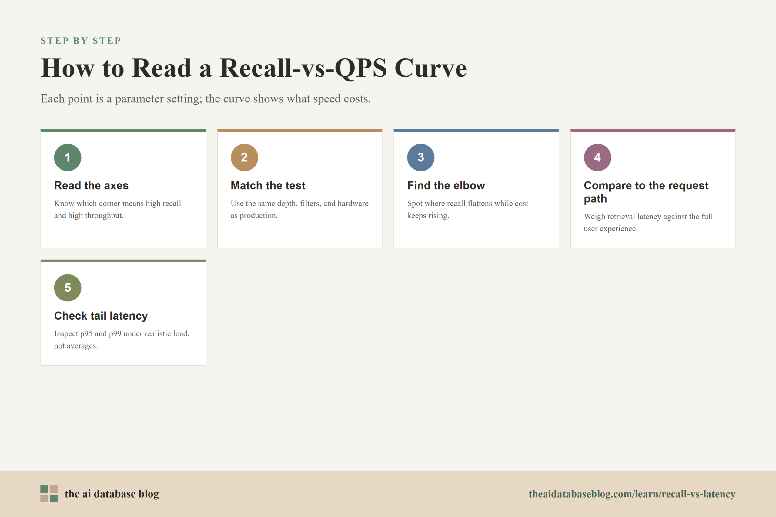
How to Read a Recall-vs-QPS Curve
A recall-versus-QPS curve shows how search quality changes as throughput changes. Usually, each point on the curve represents a different parameter setting. Points with higher QPS are faster or more efficient, but they often have lower recall. Points with higher recall usually require more search work and therefore support fewer queries per second on the same hardware.
The curve is useful because it makes the trade-off visible. Instead of asking whether an index is fast or accurate in the abstract, you can ask which setting gives the best quality within the system’s performance budget. A good curve helps you see where additional search work produces meaningful quality gains and where it mostly produces diminishing returns.
Find the Direction of Better and Worse
Start by reading the axes carefully. If recall is on the vertical axis and QPS is on the horizontal axis, the upper-right region is generally desirable because it means high recall and high throughput. In practice, most curves bend downward because higher recall costs throughput. If latency is shown instead of QPS, the desired region is usually high recall and low latency.
Make sure the curve uses the same recall depth, dataset, filters, and hardware that matter to your workload. A curve based on unfiltered vector search may be misleading if your production queries use strict metadata filters. A curve based on short vectors may not describe high-dimensional embeddings. The curve is a decision tool only when the test resembles the real workload.
Look for the Elbow
The elbow is the part of the curve where recall gains begin to flatten while cost continues to rise. Before the elbow, increasing search effort may produce large recall improvements. After the elbow, the system may spend much more time or capacity to recover only a small number of additional exact neighbors.
The elbow is often a strong candidate operating point because it balances quality and efficiency. For example, if moving from one setting to another improves recall from 80 percent to 93 percent with a modest QPS loss, that may be worthwhile. If the next step improves recall from 93 percent to 95 percent but halves QPS, the extra quality may or may not justify the cost. The answer depends on the application.
Compare Against the User Experience
The curve should be interpreted in the context of the full request path. In a RAG application, vector retrieval may be only one part of total latency. The system may also rewrite the query, apply filters, rerank documents, call a language model, stream output, and log traces. If retrieval is a small fraction of total latency, spending a few more milliseconds for better recall may be reasonable. If retrieval is already the bottleneck, the operating point may need to favor QPS.
User tolerance also varies by use case. An interactive autocomplete feature may need very low latency and accept lower recall. A legal, medical, or compliance-oriented retrieval workflow may need higher recall and tolerate more latency, while still requiring independent validation. Internal analytics may prioritize throughput for batch processing. The curve does not choose for you; it shows the cost of each choice.
Watch for Tail Latency and Saturation
A recall-versus-QPS curve can hide instability if it reports only average values. As search parameters increase, each query does more work. Under high concurrency, that extra work can create queues, cache pressure, or memory bandwidth contention. The result may be a curve point that looks acceptable in average QPS but has poor tail latency.
Before choosing a point, inspect p95 and p99 latency at realistic traffic levels. A setting is risky if it reaches the desired recall only when the system is close to saturation. In production, traffic spikes, uneven filters, larger result sets, or background indexing can push that setting over the edge.
Reading the curve well gives you a short list of candidate settings. Choosing among them requires one more step: connecting the curve to a concrete operating point and validating it with application-level tests.
How to Pick an Operating Point
An operating point is the parameter setting you choose for production or for a specific class of queries. It should reflect the minimum recall needed for useful results, the maximum latency users can tolerate, the throughput the system must support, and the infrastructure cost the team is willing to pay. The best operating point is rarely the highest-recall point on the chart. It is usually the point where quality is good enough and performance is stable.
A practical process starts with requirements. Define the result depth, target recall range, maximum acceptable p95 latency, expected QPS, dataset size, update pattern, metadata filtering needs, and available hardware. Then benchmark a small grid of parameter settings. For each point, record recall, average latency, tail latency, QPS, memory use, and any build or update cost that matters.
Start with the Smallest Useful Search Effort
Begin with conservative query-time settings and increase search effort until recall reaches a useful level. This prevents over-tuning from the start. In many systems, the first few increases in search breadth produce the largest gains. Once recall gains slow down, you can decide whether the remaining misses are important enough to justify the added cost.
This approach also helps separate query-time tuning from index rebuild decisions. If higher query-time breadth cannot reach the desired recall within the latency budget, the index structure may need to change. That could mean a denser graph, different clustering, less aggressive compression, better reranking, or a different data modeling strategy.
Use Different Settings for Different Query Types
Not every query needs the same operating point. A consumer-facing search box, an internal research tool, and a background enrichment job may have different latency and recall requirements. Some systems use lower-latency settings for interactive exploration and higher-recall settings for workflows where completeness matters more.
Adaptive tuning can also be useful. For example, filtered queries may need different settings from unfiltered queries because filters can reduce the candidate pool. Short, ambiguous queries may benefit from wider search or reranking. High-confidence queries with clear nearest neighbors may not need as much exploration. The main idea is to align search effort with query value and difficulty.
Validate with End-to-End Quality
Recall is a retrieval metric, not a complete application metric. After selecting candidate operating points, test them in the full application. In a RAG system, compare answer correctness, citation quality, hallucination rate, context relevance, and user satisfaction. In semantic search, compare click-through, success rate, reformulation rate, or human relevance judgments.
This step matters because two settings with similar recall can produce different downstream outcomes. One setting may return redundant chunks, while another returns more diverse supporting evidence. One may perform well on common queries but fail on rare terminology. The operating point should be chosen with both benchmark metrics and real task outcomes in view.
After deployment, the trade-off does not disappear. Datasets grow, embeddings change, filters become more complex, and usage patterns shift. That means recall and latency should be monitored over time rather than tuned once and forgotten.
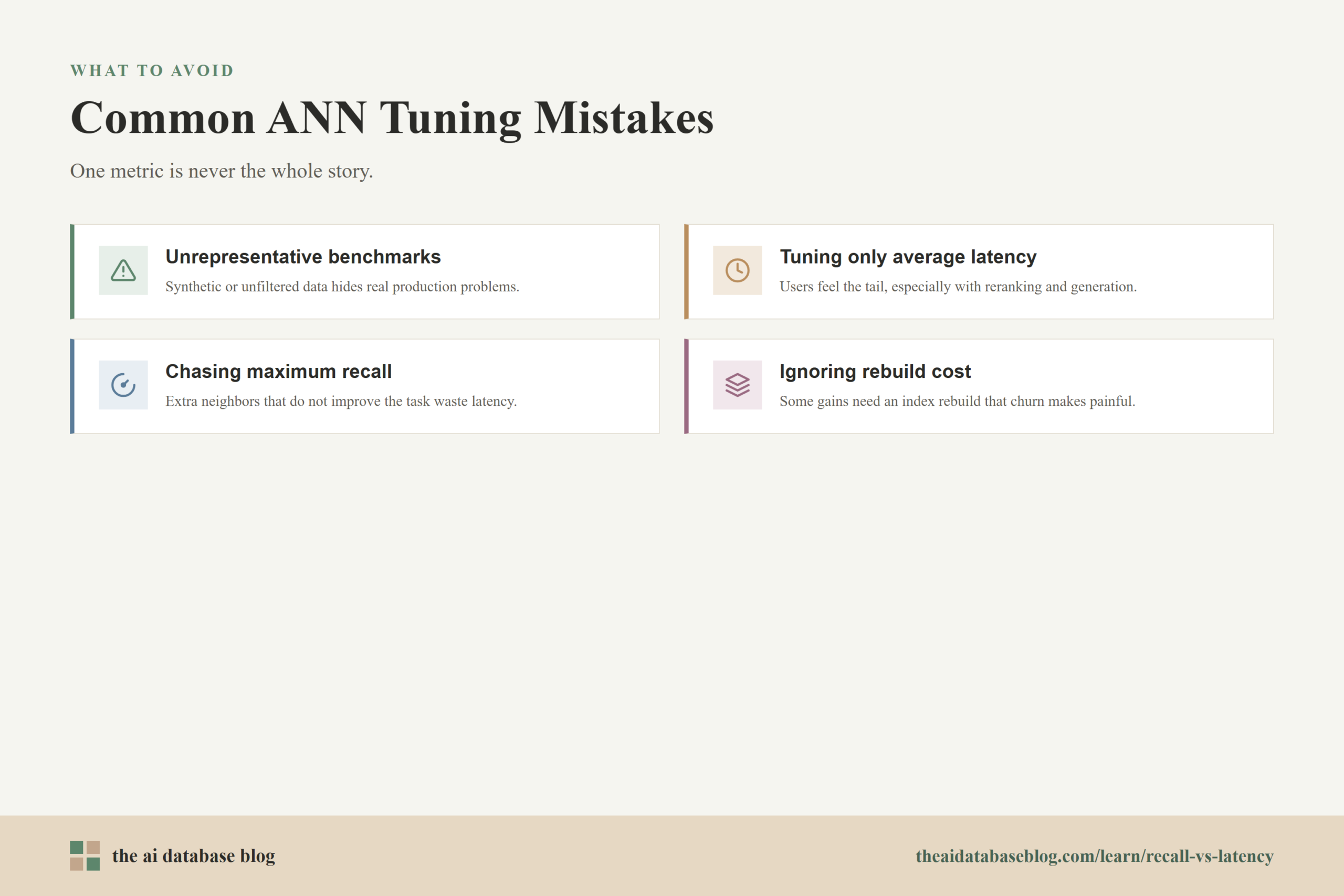
Common Mistakes When Tuning ANN Search
ANN tuning mistakes usually come from treating one metric as the whole story. High QPS is not useful if the system misses important context. High recall is not useful if the application becomes too slow or expensive to operate. A mature tuning process treats ANN search as part of a larger retrieval system with quality, latency, stability, and cost constraints.
One common mistake is benchmarking on a dataset that does not match production. Synthetic vectors, small samples, or unfiltered queries can hide problems that appear only with real embeddings, uneven metadata distributions, or long-tail user behavior. Another mistake is tuning only average latency. Tail latency is often what users notice, especially when retrieval is combined with reranking and generation.
Teams also sometimes assume that the highest recall setting is automatically best. In many applications, moving from very good recall to slightly better recall costs more than it is worth. The better question is whether the extra retrieved neighbors improve the final task. If they do not improve answers, clicks, decisions, or user trust, the added latency is probably wasted.
A final mistake is ignoring rebuild and update costs. Some parameters can be changed per query, while others require rebuilding the index or using more memory. For dynamic datasets, an index that looks excellent in a static benchmark may be difficult to maintain under frequent inserts, deletes, or embedding refreshes.
Avoiding these mistakes leads to a more balanced view of ANN performance. The goal is not to win a benchmark in isolation, but to build a retrieval layer that supports the application reliably.
Practical Example: Choosing a Setting for RAG
Consider a RAG system that retrieves 10 chunks before generating an answer. Exact search over the full corpus is too slow, so the team benchmarks an ANN index at several query-time settings. At the lowest setting, retrieval is extremely fast but recall at 10 is too low, and answer evaluation shows that important supporting chunks are often missing. At a middle setting, recall improves sharply while latency remains within the target. At the highest setting, recall improves slightly again, but QPS drops enough to create p95 latency risk during busy periods.
In this case, the middle setting is likely the best operating point. It recovers most of the relevant context, keeps retrieval within the user-facing latency budget, and leaves enough capacity for reranking and generation. The highest setting may still be useful for offline analysis, high-value queries, or workflows where completeness matters more than speed. The lowest setting may be useful for preview experiences or exploratory features where instant response matters most.
This example shows why recall-vs-QPS curves are not just benchmark charts. They help teams make product decisions. The curve explains what the system gives up and what it gains as search effort changes, while application evaluation tells you which trade-off actually serves the user.
FAQs
1. What does recall mean in ANN search?
Recall measures how many of the exact nearest neighbors were recovered by the approximate search result. If exact search would return 10 specific items and the ANN index returns 8 of them, recall at 10 is 80 percent for that query. It is a way to measure how closely approximate search matches exhaustive search.
2. Why does higher recall usually increase latency?
Higher recall usually requires the index to do more work. It may explore more graph paths, search more partitions, evaluate more candidate vectors, or rerank a larger candidate set. That extra work improves the chance of finding the same neighbors as exact search, but it also takes more time and reduces throughput.
3. Is 100 percent recall necessary for AI applications?
Not always. Some applications can perform well with less than perfect recall because the returned results are still relevant enough for the task. Other applications need very high recall because missing a key document or example creates serious quality problems. The right target depends on the use case, the result depth, and the cost of missing relevant items.
4. What is the difference between latency and QPS?
Latency is the time one query takes to return a result. QPS, or queries per second, is the number of queries the system can serve over time. They are related because slower queries usually consume more resources, but QPS also depends on concurrency, hardware, batching, and whether the system remains stable under load.
5. Which ANN parameter should be tuned first?
Query-time search breadth is often the best first parameter to tune because it directly controls the recall-latency trade-off and can usually be adjusted without rebuilding the index. Examples include graph exploration width, partition probe count, and reranking candidate count. If query-time tuning cannot meet the target, then build-time index parameters may need to change.
6. How often should ANN performance be retested?
ANN performance should be retested when the dataset grows, embeddings change, filters become more important, traffic patterns shift, or the application changes its retrieval depth. It is also useful to retest after major infrastructure changes. Recall and latency are not fixed properties of an index; they depend on the workload around it.
Takeaway
Recall and latency are connected because ANN indexes become fast by searching intelligently rather than exhaustively. Parameters control how much work the index performs, and recall-versus-QPS curves show the cost of each quality improvement. This guidance is most useful for engineers, data teams, and product builders designing vector search or RAG systems where retrieval quality and response time both matter. A practical operating point is the setting that retrieves enough useful context, stays within latency and throughput limits, and continues to perform well as the dataset and workload evolve.