HNSW and IVF are two common ways to make vector search fast without scanning every embedding. HNSW is a graph-based index that navigates through connected vectors, so it usually gives strong recall and low latency when the graph and vectors can stay in memory. IVF is a cluster-based index that partitions vectors into buckets, so it can reduce search work, support compression more naturally, and fit larger workloads more flexibly, but its recall depends on how well the clusters match the data and how many clusters are searched per query.
This guide explains how HNSW and IVF work, then compares them across speed, memory use, build time, recall, update behavior, and workload fit. By the end, you should understand why graph-based indexes often dominate in-memory high-recall search, why cluster-based indexes remain useful for large and compressed collections, and how to choose between them for AI database workloads such as semantic search, retrieval-augmented generation, recommendations, and multimodal retrieval.
What Graph-Based and Cluster-Based Indexes Are Solving
Vector search starts with embeddings, which are numerical representations of text, images, audio, code, users, products, or other objects. A query is converted into an embedding, and the database looks for stored vectors that are closest to it under a distance measure such as cosine similarity, dot product, or Euclidean distance. Exact search compares the query against every vector, which is simple and accurate but becomes expensive as the collection grows.
Approximate nearest neighbor indexes solve this by trading a controlled amount of exactness for much faster search. Instead of checking every vector, the index tries to visit only the parts of the dataset that are likely to contain good matches. The quality of the index is usually judged by latency, throughput, memory footprint, build cost, update cost, and recall. Recall measures how many of the true nearest neighbors are returned by the approximate search.
HNSW and IVF approach this problem from different directions. HNSW builds a navigable graph over the vectors. IVF divides the vector space into clusters and searches only selected clusters. Those design choices explain most of their practical behavior.
Once the goal is clear, the next question is how each index narrows the search space. HNSW narrows it by walking from neighbor to neighbor through a graph, while IVF narrows it by routing the query into a smaller set of clusters. That difference affects every operational tradeoff that follows.
How HNSW Works
HNSW stands for Hierarchical Navigable Small World. It is a graph-based index designed for approximate nearest neighbor search in high-dimensional spaces. Each vector becomes a node in a graph, and the index stores links from each node to nearby nodes. At query time, search starts from an entry point and moves through the graph toward vectors that are closer to the query.
The hierarchy is what makes HNSW efficient. Upper layers contain fewer nodes and longer-range links, helping the search move quickly toward the right region. Lower layers contain denser local connections, helping the search refine its results. This is similar in spirit to moving from a broad map to a neighborhood map before checking nearby addresses.
Three tuning ideas matter most:
- M controls how many graph neighbors each node keeps. Higher values usually improve recall but increase memory use.
- efConstruction controls how much work the index does while inserting vectors. Higher values usually improve graph quality but slow indexing.
- efSearch controls how widely the graph is explored during queries. Higher values usually improve recall but increase query latency.
Because HNSW searches by following many pointer-like graph links, it works best when the graph and the data needed for distance calculations are available in memory. If the search has to fetch graph neighbors from disk in a scattered pattern, latency can rise quickly because graph traversal tends to create random reads.
With HNSW established as a graph navigation method, IVF is easier to understand as a contrasting design. Instead of connecting every vector into a traversable graph, IVF first builds coarse regions of the vector space and uses those regions to limit the amount of data searched.
How IVF Works
IVF stands for inverted file. In vector search, an IVF index usually starts by training a coarse quantizer, often with k-means clustering or a related clustering method. The training step creates a set of centroids, which act like representatives for regions of the vector space. Each stored vector is assigned to one of these regions, also called inverted lists or buckets.
At query time, the database compares the query vector with the centroids, chooses the closest clusters, and scans vectors inside those clusters. The main query-time tuning parameter is commonly called nprobe, which means the number of clusters searched. A low nprobe value is faster but may miss relevant vectors in nearby clusters. A higher nprobe value improves recall but scans more candidates.
IVF can be used without compression, but it is often paired with compression techniques such as product quantization. That pairing is one reason IVF remains important for large vector workloads: it can reduce the number of full vectors that need to be stored or scanned in memory, and it can use a reranking step to check a smaller candidate set more accurately.
The cluster-based design also makes IVF easier to reason about in batch-oriented systems. New vectors can be assigned to existing clusters, and deleted vectors can often be marked or removed from lists. However, if the embedding distribution changes over time, the original centroids may become less representative, and the index may need retraining or rebuilding to recover quality.
Now that both indexes are defined, the useful question is not which one is universally better. The better question is which tradeoff matters most for a specific workload, because HNSW and IVF optimize different parts of the search problem.
HNSW vs IVF at a Glance
| Dimension | HNSW | IVF |
|---|---|---|
| Index type | Graph-based | Cluster-based |
| Search pattern | Best-first graph traversal through neighboring vectors | Route query to selected clusters, then scan candidates |
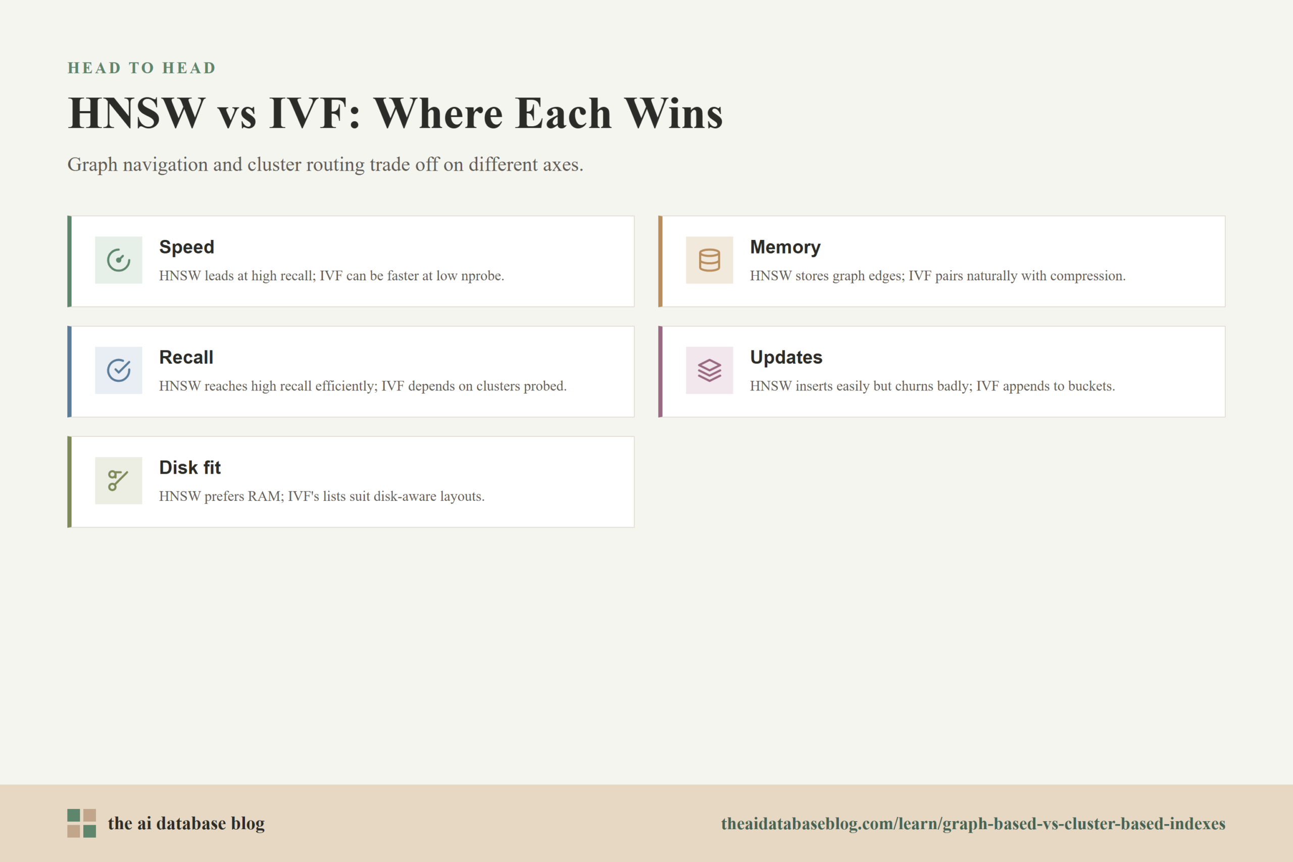
| Speed | Often very fast at high recall when memory-resident | Fast when nprobe is low or compression reduces candidate cost |
| Memory | Higher memory use because graph links add overhead | Often more memory-efficient, especially with compression |
| Build time | Can be slower because graph construction does many neighbor searches | Requires training clusters, then assigning vectors to lists |
| Recall | Typically strong at high recall targets with enough efSearch | Good when clusters are well trained and enough clusters are searched |
| Updates | Inserts are natural, deletions and heavy churn can degrade graph quality | Inserts and deletes are often simpler at the list level, but retraining may be needed as data drifts |
| Best fit | Low-latency, high-recall, memory-resident workloads | Large, compressed, batch-built, or disk-aware workloads |
The table gives the short version, but each row hides important detail. Speed, for example, is not only about raw query time. It also depends on the target recall, hardware layout, filtering needs, vector dimensionality, and whether the system can keep the working set in memory.
Speed and Query Latency
HNSW is often the faster choice when the goal is high recall at low latency and the index fits in memory. Its graph traversal can move toward promising candidates quickly without scanning large contiguous buckets. Increasing efSearch gives the search more room to explore, which usually improves recall at the cost of more distance calculations and more graph visits.
IVF speed is controlled by how many clusters are searched and how much work happens inside each cluster. When nprobe is low, IVF can be extremely fast because it scans only a small fraction of the dataset. The risk is that the nearest neighbor may sit in a cluster that was not searched. Raising nprobe improves recall but makes IVF behave more like a broader scan.
For low-to-medium recall targets, IVF can be very competitive because it avoids the overhead of graph traversal and scans compact candidate lists efficiently. For high recall targets, HNSW often has an advantage because graph navigation tends to find good candidates without needing to widen the search as dramatically.
Speed also changes when storage enters the picture. HNSW-style traversal is sensitive to random access because each step may require reading a different node and its neighbors. IVF can be more sequential because candidates are grouped in lists, which can make it easier to design around storage locality. This does not mean every IVF system is automatically disk-friendly, but the cluster layout gives system designers a useful lever.
Latency is only one side of performance. The next practical issue is memory, because many vector systems become expensive not because each query is slow, but because the index needs a large amount of RAM to stay fast.
Memory Use
HNSW usually uses more memory than IVF because it stores graph connections in addition to the vectors themselves. The graph links are the source of HNSW’s strong navigation behavior, but they are also extra index state. Increasing M improves connectivity and recall, but it also increases the number of stored edges.
In an AI database, that overhead matters because embeddings are already large. A collection with hundreds of millions of vectors can require substantial memory even before indexing overhead is added. If the workload needs high recall and low latency, the extra memory may be worth it. If cost per stored vector is the limiting factor, HNSW can become difficult to justify at very large scale unless the system uses quantization, sharding, tiering, or another memory-saving strategy.
IVF is often more memory-flexible. The cluster assignments and centroids add overhead, but the structure can pair naturally with compressed vector representations. IVF with product quantization or other compact encodings can store many more vectors in the same memory budget, although compression may reduce accuracy unless reranking is used.
The important distinction is that HNSW tends to spend memory on navigability, while IVF tends to spend structure on partitioning and can spend less memory per candidate when compression is used. That makes HNSW attractive when memory is available and latency matters most, and IVF attractive when memory pressure is a primary design constraint.
Memory decisions also affect indexing time. A richer graph can improve query quality but takes effort to construct, while a clustered index must pay the cost of training and assignment. The next section explains why build time is not just a one-time inconvenience.
Build Time and Operational Cost
HNSW builds the index incrementally by inserting vectors and connecting them into the graph. During insertion, the index searches the existing graph to find good neighbors for the new node. Higher efConstruction values usually produce better links and stronger recall, but they also make indexing slower. Build time can become significant for very large collections or frequent rebuilds.
IVF has a different build profile. It first needs a training step to learn centroids from representative data, then assigns vectors to the nearest centroid or centroids depending on the implementation. Training can be expensive when the number of clusters is large, but assignment is conceptually straightforward and can often be batched efficiently.
For static or mostly append-only datasets, both approaches can work well if the build process is planned. For frequently changing datasets, the cost of maintaining quality becomes more important than the initial build time. HNSW can accept inserts naturally, but deletes and heavy churn can leave the graph less clean. IVF can assign new vectors to existing clusters, but if the new data distribution differs from the training sample, the cluster structure can become stale.
This is why production systems often separate initial indexing from ongoing maintenance. They may use background compaction, periodic rebuilds, delta indexes, or hybrid layouts to keep search fresh without constantly rebuilding the whole structure.
Build time matters because it is connected to recall. A cheaply built index may answer quickly but miss too many relevant results. The next section looks at how HNSW and IVF reach high recall, and why they fail in different ways.
Recall and Relevance
HNSW is known for strong recall at practical latency when tuned well. Its graph structure gives the search many paths toward nearby vectors, and increasing efSearch lets it explore more candidates before returning results. This makes HNSW a common choice for retrieval systems where missing a relevant document is costly, such as RAG pipelines that need good context for generated answers.
However, HNSW recall is not automatic. It depends on parameters, data distribution, insertion order, vector dimensionality, distance metric, filtering behavior, and how much search effort is allowed. Highly clustered or uneven data can require more careful tuning. Metadata filters can also affect recall if the search finds good vector neighbors that are later filtered out, leaving too few valid candidates.
IVF recall depends heavily on the coarse clustering step. If the true nearest neighbors are in clusters that are searched, IVF can perform well. If relevant vectors are split across clusters that are not searched, recall drops. Raising nprobe reduces that risk by searching more clusters, but it increases latency and candidate scanning.
IVF with compression adds another recall consideration. Compressed distances are approximate, so the first candidate ranking may be less accurate than full-vector comparison. A common mitigation is reranking: retrieve a larger candidate set using compressed or approximate distances, then rerank the top candidates with more accurate vectors or a more exact distance calculation.
Recall is where workload intent matters. A product recommendation feed may tolerate approximate variety, while a legal, medical, or enterprise knowledge retrieval workflow may need a higher probability of finding the best matching passages. The index should be tuned against measured recall on the actual dataset, not only against default parameters.
Even a well-tuned index can lose quality if the data changes. That makes update behavior the next major design question, especially for AI applications where new documents, events, profiles, and embeddings arrive continuously.
Update Behavior
HNSW is naturally incremental for inserts because each new vector can be added by searching the graph and creating neighbor links. This is useful for systems that need new content to become searchable quickly. The harder part is deletion and replacement. Removing a node can disturb the graph structure, so many systems use soft deletion, tombstones, or background repair rather than physically rewiring the graph immediately.
Heavy update churn can create practical problems for HNSW. If many vectors are inserted, deleted, or replaced, the graph may contain stale links, uneven connectivity, or too many deleted nodes that still affect traversal. The system may need periodic rebuilds or maintenance to restore search quality and memory efficiency.
IVF updates are often simpler at the bucket level. A new vector can be assigned to a cluster and appended to its list. A deleted vector can be removed or marked inactive. That makes IVF appealing for batch updates and list-oriented storage. The deeper issue is that the centroids were trained on earlier data. If the dataset changes significantly, new vectors may be assigned to clusters that no longer represent the distribution well.
For both index families, updates are not just a data management feature. They affect relevance. A system can appear fresh because new vectors are present, but still lose recall if graph links degrade or cluster assignments become stale. Good AI database design treats freshness, recall, and maintenance cost as a combined problem.
Update behavior becomes even more important when the dataset is too large for RAM. At that point, the choice is not simply HNSW versus IVF, but which layout can minimize expensive storage access while preserving enough recall.
In-Memory vs Disk-Based Workloads
HNSW is best understood as an in-memory-first index. Its graph traversal pattern works beautifully when neighbor lists and vector data can be accessed quickly. For collections that fit comfortably in RAM, HNSW can offer an excellent balance of speed and recall, especially for interactive search, RAG retrieval, personalization, and other latency-sensitive AI workloads.
HNSW becomes more challenging when the graph or vectors must live primarily on disk. Graph search tends to jump from node to node, which can turn into many random reads. Disk-oriented graph indexes exist, but they usually modify the graph layout, store compressed representations in memory, use beam search, or carefully organize disk pages to reduce random I/O. In other words, disk-friendly graph search is not just ordinary HNSW placed on an SSD.
IVF is often a better conceptual fit for disk-aware or memory-constrained workloads because vectors are grouped into lists. A query can select a limited number of lists and scan them, which is easier to align with block reads, compression, and candidate reranking. IVF-based systems can also keep centroids or compressed codes in memory while storing larger candidate data elsewhere.
That said, IVF is not automatically better for every disk-based workload. If high recall is required, the system may need to probe many clusters, which can increase I/O and latency. Disk-based vector search is usually best handled by an index specifically designed for storage hierarchy, whether it is graph-based, cluster-based, or hybrid.
A practical rule is simple: choose HNSW when the hot working set fits in memory and high recall matters; consider IVF or a hybrid approach when memory footprint, compression, batch construction, or disk locality matters more. For billion-scale systems, the best design often combines ideas from both families rather than using a textbook version of either.
With the in-memory and disk tradeoffs in place, the final decision can be reduced to a few workload questions. The next section turns the comparison into a practical selection guide.
How to Choose Between HNSW and IVF
Choose HNSW when your workload needs high recall, low latency, and enough memory is available to keep the index fast. It is especially strong when the dataset is large enough that exact search is too slow, but not so large that graph memory dominates infrastructure cost. It is also a good default for many RAG and semantic search systems because missed nearest neighbors can directly reduce answer quality.
Choose IVF when you need a more compact, batch-friendly, or compression-friendly index. IVF is useful when you can tolerate tuning nprobe, reranking candidates, and measuring the recall-latency tradeoff carefully. It can also be a strong choice when the dataset is very large, when memory is limited, or when the storage layout benefits from scanning grouped candidates rather than following graph links.
Use these questions to guide the decision:
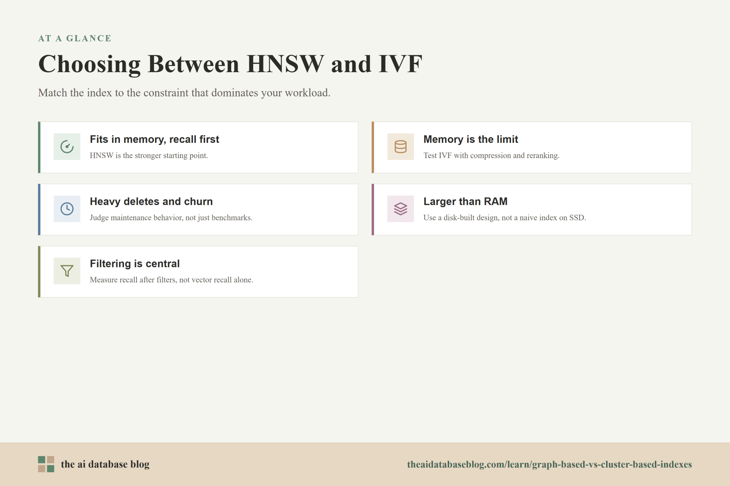
- If the index and vectors fit in memory and search quality is the top priority, HNSW is usually the stronger starting point.
- If memory cost is the limiting factor, IVF with compression is often worth testing.
- If updates are frequent but mostly inserts, both can work, with HNSW providing direct insertion and IVF providing cluster assignment.
- If deletes, replacements, and churn are heavy, evaluate maintenance behavior rather than only initial benchmark results.
- If the dataset is larger than memory, prefer a design built for disk or hybrid memory and disk access, not a naive in-memory index moved onto SSD.
- If metadata filtering is central, test recall after filtering, because vector-only recall can overstate real application quality.
The safest production answer is to benchmark both against the actual embeddings, filters, query mix, and recall target. HNSW and IVF can both look excellent in simple benchmarks and behave differently once real metadata filters, update patterns, skewed data, and storage limits appear.
Common Use Cases
For a document retrieval system that supports RAG, HNSW is often a strong default when the corpus fits in memory. The system benefits from high recall because the language model depends on retrieved context. If the index misses the best passages, the generated answer may become less grounded even if latency is low.
For a large media, recommendation, or product catalog where memory cost is a major constraint, IVF may be attractive. The system can use clustering to narrow the search and compression to reduce storage. A reranking stage can then improve precision on a smaller candidate set.
For a fast-changing event or content stream, neither index should be chosen only by query speed. The design should account for update freshness, deletion handling, rebuild cost, and whether stale graph links or stale centroids will reduce quality over time. In many systems, a small fresh index for recent data and a larger optimized index for stable data can work better than forcing one index to do everything.
These examples show why the right index is tied to the full retrieval architecture. The index is not just a data structure; it shapes latency, cost, freshness, and relevance across the application.
FAQs
1. Is HNSW always faster than IVF?
No. HNSW is often faster at high recall when the index is memory-resident, but IVF can be faster at lower recall targets or when it scans a small number of clusters. IVF can also benefit from compression and efficient sequential scanning. The real answer depends on recall target, vector dimension, hardware, filtering, and tuning.
2. Which index has better recall?
HNSW often reaches high recall more efficiently because graph traversal can explore promising neighborhoods without scanning many broad partitions. IVF can also achieve good recall, but it usually needs enough clusters to be searched with nprobe and may need reranking when compression is used. Both should be evaluated on the actual workload.
3. Why does HNSW use more memory?
HNSW stores graph links for each vector in addition to the vector data. Those links make the graph navigable, but they add overhead. Increasing the number of neighbors per node can improve recall, but it also increases memory consumption.
4. Why is IVF often paired with product quantization?
IVF reduces the search space by selecting clusters, while product quantization reduces the storage and comparison cost of vectors inside those clusters. Together, they can make large vector collections more memory-efficient. The tradeoff is that compressed comparisons are approximate, so systems often rerank a candidate set with more accurate data.
5. Which index handles updates better?
It depends on the type of update. HNSW handles inserts naturally, but deletions and heavy churn can require tombstones, repair, or rebuilds. IVF can append new vectors to clusters and mark deleted vectors more simply, but its centroids may become stale if the data distribution changes. Both need maintenance planning for dynamic workloads.
6. Which index is better for disk-based vector search?
Plain HNSW is usually better suited to memory because graph traversal can cause random access. IVF can be easier to adapt to disk-aware layouts because vectors are grouped into lists, but high recall may require probing many lists. Large disk-based systems often use specialized or hybrid designs rather than simply moving a standard in-memory index to SSD.
Takeaway
HNSW and IVF both speed up vector search by avoiding a full scan, but they do it in different ways: HNSW navigates a graph, while IVF searches selected clusters. HNSW is usually the stronger choice for memory-resident workloads that need low latency and high recall, such as RAG retrieval over a corpus that fits in RAM. IVF is often better when memory efficiency, compression, batch indexing, or disk-aware access patterns matter more. For engineers and AI database practitioners, the practical lesson is to choose based on measured recall, latency, memory, build cost, update behavior, and storage layout rather than treating either index as universally best.