Filtered approximate nearest neighbor search is the problem of finding the most similar vectors while also honoring metadata constraints such as tenant, language, date, product category, region, permission, or document type. Filtering breaks naive ANN because the index was usually built to navigate the full vector space, not the smaller subset that remains after a filter is applied. When the filter is selective, the search can fall off a recall cliff: the algorithm may quickly find nearby vectors that do not match the filter, discard them, and return too few or lower-quality results. High-recall filtered ANN systems avoid this by bringing the filter into query planning, index traversal, candidate generation, partitioning, or exact fallback instead of treating filtering as a simple afterthought.
This guide explains why filtered ANN is harder than ordinary vector search, what the recall cliff looks like in practice, and which algorithmic approaches help preserve recall under metadata constraints. It focuses on the database and retrieval design choices that matter when semantic search needs to obey structured rules, especially in retrieval-augmented generation, recommendation, personalization, and access-controlled search systems.
What Filtered ANN Search Means
Approximate nearest neighbor search is designed to avoid scanning every vector in a dataset. Instead of comparing a query vector against every stored vector, an ANN index uses a structure such as a graph, partitioned index, quantized representation, or tree-like layout to quickly find candidates that are likely to be close. The word approximate matters because the system trades a small amount of recall for much lower latency and cost.
Filtered ANN adds a second condition to the query. The result must be close to the query vector and must satisfy a structured predicate. A query might ask for the top 10 semantically similar support articles where the language is English, the product is “billing,” the document is not archived, and the requesting user is allowed to see it. The search is no longer just a vector similarity problem. It becomes a combined vector and structured-data retrieval problem.
The difficulty is that vector similarity and metadata constraints do not always align. The nearest vectors in the full dataset may belong to the wrong tenant, fall outside a date range, or be hidden by permissions. If the ANN algorithm spends most of its work visiting those ineligible vectors, the search can look fast while producing weak or incomplete results.
Once filtering is understood as part of the search problem rather than a cleanup step, the next question becomes why a simple approach often fails. The answer starts with how ANN indexes navigate data.
Why Filtering Breaks Naive ANN
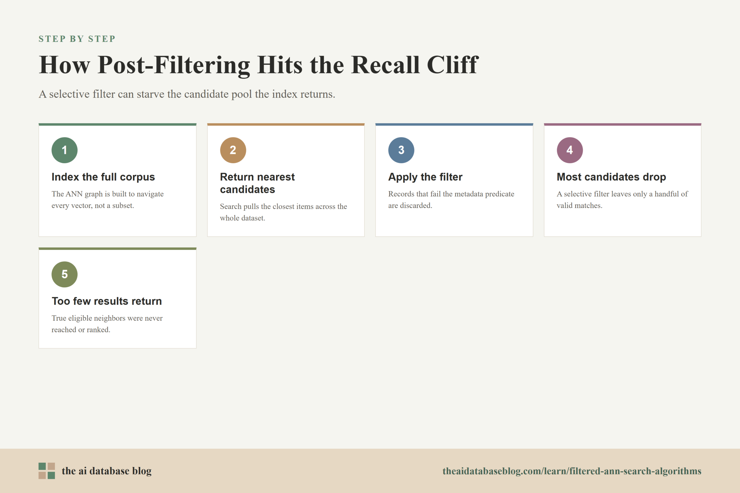
Naive filtered ANN usually means running ordinary ANN first and then applying the metadata filter to the returned candidates. This is often called post-filtering. It is simple to implement because the vector index does not need to understand metadata. The search asks the index for a candidate pool, removes anything that does not match the filter, and returns the remaining nearest items.
This approach works when the filter is broad. If 80 percent of the corpus matches the filter, many of the nearest candidates found by the ordinary ANN search are likely to survive. The trouble begins when the filter is selective. If only 1 percent of the corpus matches, the first 100 approximate candidates may contain very few valid results, even if the correct filtered neighbors exist elsewhere in the index.
The problem is especially visible in graph-based ANN indexes such as HNSW-like or DiskANN-style structures. These indexes search by walking through neighbors that are close in vector space. If the search is allowed to walk through all nodes but only return filtered nodes, it may waste work evaluating ineligible candidates. If the search is allowed to walk only through filtered nodes, the graph may become poorly connected because edges were created for the full dataset, not for each filtered subset.
Filtering can also break assumptions inside partitioned indexes. A clustering or inverted-file index may route the query to a few vector partitions that are promising for the full dataset. But after the filter is applied, those partitions may contain too few eligible records, while another partition with more valid filtered results is never searched. The result is not just lower recall; it is unstable recall that changes sharply with filter selectivity, data distribution, and the correlation between metadata and vector position.
This instability is what makes filtered ANN more than a tuning problem. Increasing a search parameter may help, but it does not always fix the structural mismatch between a full-corpus index and a filtered result set.
The Recall Cliff
The recall cliff is the sharp drop in result quality that happens when a filter becomes selective enough that ordinary ANN candidate generation no longer reaches enough eligible neighbors. Recall measures how many of the true nearest filtered results appear in the returned result set. In an unfiltered query, a well-tuned ANN index might retrieve most of the true top results. Under a selective metadata filter, the same index settings can suddenly return only a small fraction of the true filtered nearest neighbors.
A simple example makes the failure mode easier to see. Suppose a database stores 10 million document chunks, and a query asks for the top 10 most relevant chunks that belong to one customer account. If that customer owns only 20,000 chunks, the filter keeps 0.2 percent of the corpus. A post-filtered ANN search that retrieves 200 candidates from the full corpus may statistically see very few candidates from that customer unless the customer-specific chunks are unusually concentrated near the query. The valid answers may exist, but the search did not explore deeply enough to find them.
The cliff is not caused only by low selectivity. It can also appear when metadata and vector space are poorly correlated. A language filter may align with embedding clusters if texts in different languages occupy different regions. A permission filter or tenant filter may be almost random with respect to vector similarity. Random-looking filters are harder because the nearest valid points can be scattered across the graph or across many partitions.
Another cause is candidate starvation. The system may ask the ANN index for the top 100 approximate candidates, but after filtering only three remain. If the application requires 10 results, the database must either return too few results, lower relevance quality, retry with a larger candidate pool, or switch strategies. This retry behavior can make latency unpredictable because hard filtered queries require repeated or deeper searches.
The practical lesson is that filtered ANN needs to be evaluated separately from ordinary ANN. A system can have strong unfiltered recall and still fail filtered workloads if the query planner, index layout, and traversal strategy do not account for metadata constraints.
Because the recall cliff comes from the interaction between filters and candidate generation, the strongest solutions change how candidates are found in the first place. The main approaches differ in where they place the filter: before search, after search, inside search, inside the index, or inside the planner.
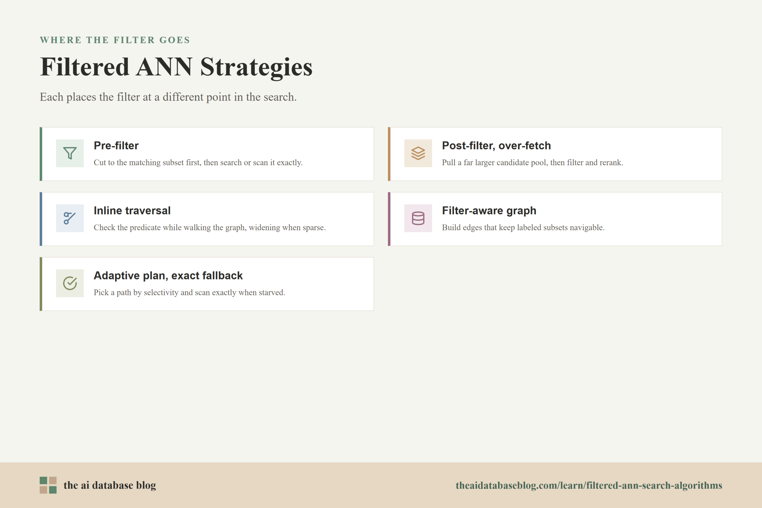
Approach 1: Pre-Filtering Before Vector Search
Pre-filtering applies the structured predicate first, then performs vector search only over the matching subset. Conceptually, this is the cleanest model because the vector search sees exactly the filtered dataset. If the filtered subset is small enough, the system can even compute exact distances over all matching records and avoid ANN error entirely.
The advantage of pre-filtering is correctness. The search is not distracted by ineligible records, and the returned neighbors are compared within the right population. This can work well for highly selective filters, access-control predicates, or tenant-specific searches where the matching set is small enough to scan or to search with a small dedicated index.
The disadvantage is cost and index management. If the system needs fast ANN over many possible filters, it cannot build a separate vector index for every combination of metadata values. A product catalog might support filters for category, price range, brand, availability, region, and user segment. The number of possible filtered subsets grows quickly, and most subsets change over time as records are inserted, updated, or deleted.
Pre-filtering also depends on a reliable estimate of the filtered set size. If the filter returns 500 records, exact search may be excellent. If it returns 5 million records, exact search may be too slow, and building an ad hoc ANN index at query time is usually impractical. This is why production systems often combine pre-filtering with query planning rather than use it as the only strategy.
Pre-filtering shows that the ideal filtered search space is often smaller than the whole corpus. The next approach takes the opposite position: keep the existing ANN index untouched and try to recover enough valid results after the fact.
Approach 2: Post-Filtering With Over-Fetching
Post-filtering runs ANN over the full dataset, collects more candidates than the final top-k, and then filters and reranks those candidates. The common improvement over naive post-filtering is over-fetching: instead of asking for 10 candidates to produce 10 results, the system might ask for 100, 1,000, or a dynamically chosen number based on expected filter selectivity.
This approach is attractive because it works with ordinary ANN indexes. It does not require a filter-aware graph, partition layout, or special metadata structure. It is also useful when filters are broad, when filtered queries are rare, or when the application can tolerate occasional retries for difficult filters.
The weakness is that over-fetching scales poorly as filters become more selective. If only 0.1 percent of the corpus matches, the system may need to retrieve thousands or tens of thousands of candidates to reliably find 10 eligible results. That can erase the latency benefit of ANN while still failing on unlucky queries where the valid neighbors are not reached by the initial search path.
Post-filtering also creates a subtle relevance issue. The candidate pool is optimized for unfiltered nearest neighbors, not filtered nearest neighbors. A valid item that is the best answer within the filtered subset may rank far outside the top candidates in the full corpus. Unless the system searches very deeply, that item will never be considered.
Over-fetching is therefore a reasonable baseline, not a complete solution. It becomes stronger when paired with adaptive query planning, iterative search, or a fallback that detects candidate starvation before returning a poor result set.
Approach 3: Inline Filtering During ANN Traversal
Inline filtering brings metadata checks into the ANN search process itself. Instead of searching first and filtering later, the algorithm uses the filter while exploring candidates. In a graph index, this might mean checking whether each visited node matches the predicate, deciding whether it can be returned, and deciding whether it should be used to continue traversal.
There are two important design choices here. The first is whether non-matching nodes can be used as stepping stones. If the search completely refuses to traverse through non-matching nodes, it may get trapped because the filtered subgraph is not navigable. If it can traverse through non-matching nodes but only return matching nodes, it has a better chance of reaching good filtered results, but it may spend extra work on records that cannot be returned.
The second design choice is how aggressively the search expands when filtered results are sparse. A filter-aware traversal can widen the search frontier, use multiple entry points, continue beyond the normal stopping condition, or adjust the candidate queue based on how many valid results have been found. These tactics help avoid returning early when the unfiltered nearest region contains too few eligible records.
Inline filtering is often a good fit when the system needs one shared index but must support many dynamic predicates. It avoids the explosion of per-filter indexes while doing more than simple post-filtering. Its main challenge is tuning. If the traversal is too strict, recall drops. If it is too broad, latency rises. The best behavior depends on selectivity, metadata distribution, and how expensive it is to check filters and fetch records.
Inline filtering improves query-time behavior, but it still relies on an index that may have been built without knowledge of the metadata. A deeper solution is to change the index so filtered subsets remain easier to navigate.
Approach 4: Filter-Aware Graph Indexes
Filter-aware graph indexes build metadata awareness into the structure of the ANN graph. In ordinary graph ANN, edges connect vectors that are useful for navigating the vector space. In filter-aware graph construction, edges can also be chosen to preserve navigability for filtered searches. The goal is to make sure that when a query restricts results to a label or metadata condition, the eligible nodes are still reachable through useful paths.
One common idea is to add or preserve edges that connect points sharing filter labels. Another is to stitch together subgraphs so that each important filtered subset has enough internal connectivity. This reduces the chance that a search gets stuck outside the valid subset or fails to discover eligible candidates near the query.
The benefit is high recall at interactive latency for filters that are important enough to influence index design. This is especially valuable when filters are common, predictable, and business-critical, such as language, region, customer segment, or access tier. A filter-aware graph can avoid the worst recall cliff because the graph is no longer purely optimized for unfiltered navigation.
The cost is complexity. Filter-aware graph construction can increase build time, memory use, and maintenance work. It may be harder to support frequent metadata updates, range filters, high-cardinality fields, or arbitrary combinations of predicates. A graph designed around one label model may not generalize cleanly to all future filters.
Filter-aware graphs are powerful when the workload is known and the filtered dimensions are stable. When filters are more varied or when the system needs flexible structured querying, partition-based and planner-based approaches become more important.
Approach 5: Partitioning, Sharding, and Per-Segment Search
Partitioning divides the corpus into smaller units before or during vector search. Some partitions are based on vector similarity, some on metadata, and some on a combination of both. The search planner then chooses which partitions to scan or probe for a particular query and filter. This can reduce wasted work because the system avoids searching parts of the corpus that are unlikely or impossible to contain valid results.
Metadata partitioning works well when a filter has natural boundaries. Tenant-specific data, language-specific data, geographic regions, and document collections are common examples. If the query is scoped to a tenant, the database can search that tenant’s partition instead of the entire corpus. This can improve recall because the ANN search is operating over a population closer to the filtered ground truth.
Vector partitioning can also help, especially when paired with enough probing. An inverted-file style index routes a query to nearby clusters. Under filters, the system may need to probe more clusters than it would for unfiltered ANN because the nearest clusters may not contain enough eligible records. Partition-based methods can perform well for some filtered workloads because they make it natural to widen or narrow the searched portion of the dataset.
The tradeoff is skew. Some partitions may be huge, while others are tiny. Some filters may align with partitions, while others cut across many of them. If the partition strategy is too rigid, the system can create hot spots, uneven recall, or too many small indexes to manage. Good partitioning requires workload awareness and regular monitoring as data changes.
Partitioning helps control where search happens. The remaining question is how the database decides which strategy to use for each query, because no single algorithm is best for every filter.
Approach 6: Adaptive Query Planning and Hybrid Exact Fallback
Adaptive query planning treats filtered ANN as a query optimization problem. Instead of forcing every query through the same path, the system estimates filter selectivity, expected candidate availability, index cost, and required recall. It can then choose between exact scan over the filtered subset, ANN with inline filtering, ANN with over-fetching, partition probing, or a hybrid plan that starts approximate and falls back when candidate starvation is detected.
This is often the most practical production pattern because filtered workloads are uneven. A broad query over recent English documents may work well with ordinary ANN plus a small amount of over-fetching. A narrow permission-filtered query over a few hundred records may be better served by exact search. A mid-selectivity query may need inline filtering with a larger search frontier. The right plan depends on the data and the query, not on a fixed rule.
Hybrid exact fallback is especially useful for protecting recall. If the approximate search does not find enough eligible candidates, or if the planner predicts that exact search over the filtered subset is cheap enough, the system can compute exact distances for the filtered records. This avoids returning a weak result just because the ANN path was unlucky.
The hard part is estimation. The planner needs reliable metadata statistics, cardinality estimates, and feedback from previous queries. It also needs to understand the cost of fetching vectors, checking predicates, expanding a graph frontier, probing partitions, and reranking candidates. Poor estimates can choose a fast but low-recall plan when a slightly different plan would have been both accurate and affordable.
Adaptive planning is where AI database behavior starts to look more like traditional database query optimization. The vector index is still central, but structured predicates, data distribution, and execution cost become first-class concerns.
Approach 7: Multi-Index and Workload-Aware Designs
Some systems maintain multiple indexes or auxiliary structures for different slices of the workload. Instead of relying on one universal index, they keep a main vector index plus smaller indexes, metadata bitmaps, posting lists, per-segment indexes, or specialized structures for high-value filters. At query time, the system chooses the structure that best matches the filter.
This can preserve recall because important filtered subsets receive their own search support. For example, a system with heavy tenant-scoped search might maintain tenant-level partitions or indexes for large tenants while using shared indexes for smaller tenants. A system with frequent date filters might maintain time-based segments so recent-only search does not have to fight the full historical corpus.
The benefit is workload fit. If most queries follow a small number of patterns, a multi-index design can offer high recall and predictable latency. It can also reduce the need for extreme over-fetching because the search begins closer to the eligible population.
The drawback is operational overhead. More indexes mean more memory, storage, build time, update logic, and consistency management. If metadata changes frequently, auxiliary structures must be updated correctly. If the workload shifts, indexes that once helped may become less useful. Multi-index systems are best when the database can measure query patterns and invest resources where they meaningfully improve retrieval quality.
These algorithm families are not mutually exclusive. The strongest filtered ANN systems usually combine several of them, using the query planner to decide when each one should be active.
How to Keep Recall High Under Metadata Constraints
High-recall filtered ANN starts with accepting that filter selectivity is part of the retrieval problem. The system should not measure only unfiltered recall and assume filtered queries will behave the same way. It should test filters that resemble real application constraints, including tenant filters, permission filters, range filters, category filters, and combinations of multiple predicates.
The first practical step is to track candidate survival. For each filtered query, measure how many ANN candidates were retrieved, how many matched the filter, how many were needed for the final top-k, and whether a retry or exact fallback occurred. If many queries retrieve large candidate pools but return few valid results, the system is near the recall cliff.
The second step is to tune search effort based on selectivity. Broad filters can often use ordinary ANN settings. Selective filters need larger candidate pools, wider graph traversal, more partition probes, or exact search over the filtered subset. A fixed candidate count is rarely ideal across all filters because the number of surviving candidates can vary by orders of magnitude.
The third step is to make metadata statistics available to the planner. The database should know how many records match common predicates, whether fields are high-cardinality or low-cardinality, and whether filters are correlated with vector partitions. Without this information, the planner is guessing.
The fourth step is to preserve exactness where it matters. Permission filters, tenant boundaries, compliance constraints, and user-specific visibility rules should not be approximate. ANN may be approximate in similarity, but the filter itself must be enforced exactly. The system can approximate which eligible vectors are nearest, but it should not return ineligible vectors or leak restricted records.
The final step is to benchmark filtered recall directly. Use filtered ground truth: compute the exact top-k within the filtered subset, then compare the ANN result to that set. This reveals whether the system is finding the right neighbors under the same constraints the application will use in production.
With those practices in place, algorithm selection becomes easier. The best approach depends less on abstract algorithm popularity and more on the shape of the workload.
Choosing the Right Filtered ANN Strategy
The right filtered ANN strategy depends on selectivity, update frequency, metadata cardinality, latency goals, and recall requirements. A small, highly filtered subset often favors exact search after pre-filtering. A broad filter may work well with ANN plus light post-filtering. A mid-selectivity workload with dynamic predicates may need inline filtering and adaptive search expansion. A workload with stable, frequent filters may justify filter-aware indexes or partitioned layouts.
For RAG systems, access control and recency filters deserve special attention. A retriever that returns semantically relevant but unauthorized chunks is not acceptable. A retriever that ignores recency constraints may answer from stale documentation. These filters are not just user preferences; they define the valid knowledge base for the query.
For recommendation and personalization systems, metadata constraints often express business rules. Availability, geography, language, maturity rating, price range, and inventory state can all determine whether a result is usable. In these cases, filtered recall affects both relevance and product correctness.
For multi-tenant systems, tenant filters can be difficult because they may be high-cardinality and poorly correlated with vector space. A shared graph may navigate through many tenants before finding enough eligible results for one tenant. Large tenants may deserve dedicated partitions or indexes, while smaller tenants may share infrastructure with exact fallback for narrow queries.
A useful rule is to begin with the simplest strategy that preserves recall for the actual workload, then add complexity only where measurements show a failure. Over-fetching may be enough for broad filters. Adaptive fallback may be enough for selective filters. Filter-aware graph construction or multi-index designs become worthwhile when filtered queries are frequent, latency-sensitive, and too large for exact search.
The final piece is evaluation. Without filtered recall tests, it is easy to mistake fast approximate results for good retrieval.
How to Evaluate Filtered ANN Quality
Filtered ANN evaluation should compare the system’s returned results against the exact nearest neighbors within the filtered subset. This is different from ordinary ANN evaluation against the full corpus. A result that is excellent globally may be irrelevant to the filtered ground truth if it violates the predicate or displaces a closer eligible item.
The most important metric is filtered recall at k. To compute it, first apply the metadata filter to the dataset, compute the exact top-k nearest vectors inside that subset, and then measure how many of those exact filtered neighbors appear in the approximate result. This exposes the quality loss caused by the interaction between ANN and filtering.
Latency should be measured alongside recall, not separately. A system can maintain high recall by searching extremely deeply, but that may not meet application requirements. Track median latency, tail latency, retry frequency, fallback frequency, and the number of distance computations or filter checks per query.
It is also useful to evaluate by filter selectivity buckets. For example, compare recall and latency when filters match more than 50 percent of the corpus, 10 to 50 percent, 1 to 10 percent, 0.1 to 1 percent, and less than 0.1 percent. The recall cliff often appears only in the lower-selectivity buckets, so averages can hide the failure.
Finally, evaluate combinations of filters, not just single fields. Real queries often combine tenant, permission, language, date, and document type. Each additional predicate changes the effective dataset and may make candidate starvation more likely.
FAQs
1. What is filtered ANN search?
Filtered ANN search finds approximate nearest neighbors while enforcing metadata constraints. Instead of asking only “which vectors are closest to this query,” it asks “which vectors are closest among the records that match this filter.” This is common in AI databases because applications often need semantic relevance and structured constraints at the same time.
2. Why does post-filtering reduce recall?
Post-filtering reduces recall because the ANN index retrieves candidates from the full corpus before the metadata filter is applied. If many of those candidates do not match the filter, they are discarded. The true nearest eligible records may never enter the candidate pool, especially when the filter is selective or poorly correlated with vector similarity.
3. What is the recall cliff in filtered vector search?
The recall cliff is the sudden drop in filtered result quality when a metadata constraint becomes selective enough that the ANN search no longer finds enough eligible candidates. It often appears when candidate pools are too small, graph traversal cannot reach filtered nodes efficiently, or the index probes too few partitions under the filter.
4. Is pre-filtering always better than post-filtering?
Pre-filtering is often more accurate because it searches only the eligible subset, but it is not always faster or easier to operate. If the filtered subset is small, exact search after pre-filtering can be excellent. If the subset is large or if there are many possible filter combinations, pre-filtering may require expensive scans or too many indexes.
5. How do filter-aware graph indexes help?
Filter-aware graph indexes add metadata awareness to graph construction or traversal so filtered subsets remain easier to navigate. They can add edges among records that share labels, preserve paths through filtered regions, or use filter-aware entry points. This helps the search find eligible neighbors without relying only on over-fetching from the full corpus.
6. What is the best way to evaluate filtered ANN?
The best evaluation is filtered recall at k, measured against exact nearest neighbors inside the filtered subset. The benchmark should include realistic metadata predicates, combinations of filters, selectivity buckets, and latency measurements. This shows whether the system keeps recall high under the same constraints the application will use in production.
Takeaway
Filtered ANN search is difficult because metadata constraints change the effective search space while many ANN indexes are built to navigate the full vector space. Naive post-filtering can work for broad filters, but selective filters can create a recall cliff where the system returns too few or lower-quality eligible results. The most reliable AI database designs use a mix of pre-filtering, inline filtering, filter-aware traversal, partitioning, adaptive planning, and exact fallback to keep recall high. This guidance is most useful for engineers and technical decision-makers building RAG, recommendation, personalization, or multi-tenant search systems where vector similarity must obey metadata rules such as permissions, tenant boundaries, language, date, or product category.