Cost optimization for vector search starts with understanding what the system is really paying for: memory to keep vectors and indexes available, compute to run approximate nearest neighbor search, query volume that drives read work, and ingestion work that creates or updates embeddings. The most effective savings usually come from reducing vector size, choosing the right index and deployment model, separating hot data from cold data, sizing capacity around measured traffic, and avoiding unnecessary re-embedding when documents or models change.
This guide explains the main cost drivers behind vector search and shows how teams can control them without blindly lowering quality. It covers memory, compute, queries, quantization, tiered storage, right-sizing, serverless versus provisioned infrastructure, and practical ways to reduce the cost of re-embedding content in AI database and retrieval-augmented generation systems.
Why Vector Search Costs Add Up
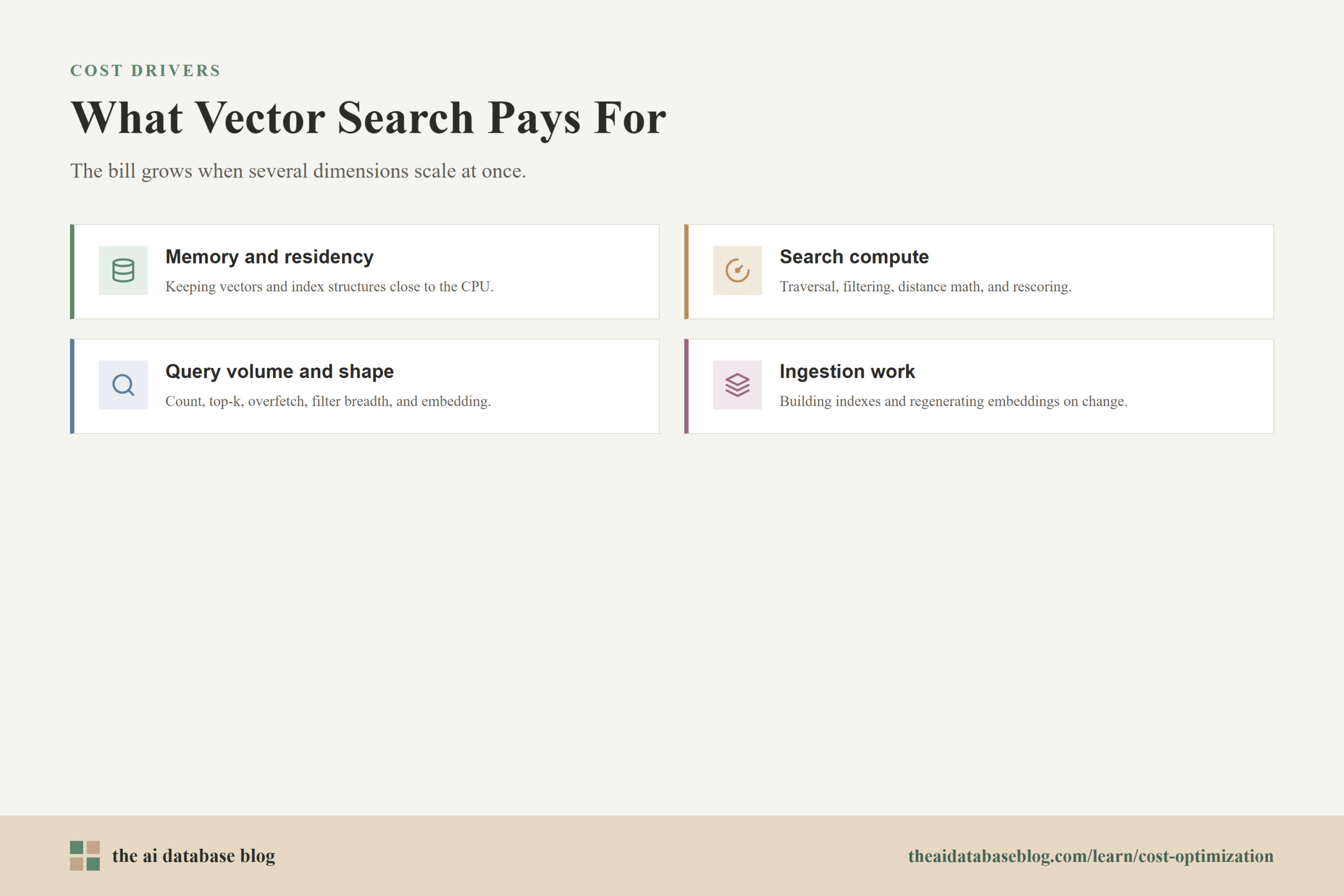
Vector search looks simple from the application side: send a query vector, retrieve the nearest items, and pass the best results into an application or AI workflow. Behind that request, however, the database may need to maintain millions or billions of high-dimensional vectors, keep an index structure available, apply metadata filters, compute similarity scores, and return enough candidates to support accurate ranking. Each of those steps consumes infrastructure, and the bill grows when the workload scales in more than one direction at once.
The first source of cost is storage, especially when vectors are stored as full-precision numbers. A 768-dimensional vector stored as 32-bit floating point values uses less space than a 3,072-dimensional vector, but both become expensive at large scale once index overhead, metadata, replication, and operational headroom are included. The second source is compute, because approximate nearest neighbor search still needs distance calculations, graph traversal, filtering, and sometimes rescoring. The third source is traffic: frequent queries, high top-k values, broad filters, and bursty usage can increase read work even when the stored dataset stays the same.
These costs are tightly connected. A larger embedding model can improve retrieval quality in some systems, but it also increases memory and storage. A more accurate index configuration can improve recall, but it may need more RAM or CPU. A broader query can find better candidates, but it may scan more of the index. Good cost optimization is therefore not just about spending less; it is about choosing the cheapest configuration that still meets the application’s retrieval-quality and latency requirements.
Once the basic cost shape is clear, the next question is where the largest bill pressure usually comes from. In most production systems, that means looking first at memory, compute, and query patterns before changing more subtle parts of the stack.
Main Cost Drivers: Memory, Compute, and Queries
The main cost drivers in vector search are not mysterious, but they are easy to underestimate during prototyping. A small demo may store a few thousand vectors and run a handful of searches per day. A production AI application may store every document chunk, product description, support article, message, profile, or event as an embedding, then search that corpus for every user request. The same architecture that felt inexpensive in development can become costly when vector count, dimensionality, concurrency, and update frequency all rise together.
Memory and Vector Residency
Memory is often the largest cost driver because many vector search systems perform best when vectors, compressed representations, or index structures are kept close to the CPU. Even when full vectors are stored on disk, the system may keep graph links, compressed codes, filter structures, or candidate data in memory to preserve low latency. Replication and high availability multiply that footprint because the same index may exist on more than one node.
The practical questions are: how many vectors must be searchable now, how many dimensions each vector has, what precision is required, how much index overhead is added, and how many replicas are needed. Reducing any one of those variables can lower cost, but each reduction should be tested against retrieval quality and response time.
Compute for Search, Filtering, and Rescoring
Compute cost comes from the work needed to locate nearest neighbors quickly enough for the application. Approximate search methods reduce the need to compare a query against every vector, but they still perform graph traversal, candidate generation, metadata filtering, and distance calculations. If the system overfetches candidates and then reranks them with full-precision vectors or another model, compute usage rises again.
Compute also appears during writes. Building or updating an index is not free, especially when large batches of vectors are added, deleted, or refreshed. Systems with frequent ingestion need to budget for both read-side search work and write-side maintenance work.
Query Volume and Query Shape
Query cost is not only about the number of requests. A million narrow searches with a small top-k can cost less than fewer searches that ask for many candidates, use broad filters, or search across multiple namespaces. Query embedding can also add cost when every search request must first be converted into a vector.
Teams should track query count, top-k, candidate overfetch size, filter selectivity, latency target, and cache hit rate together. A high-volume system with predictable traffic may need a different cost strategy than a low-volume system with unpredictable spikes.
After the core cost drivers are visible, the most direct optimization is usually to reduce the memory footprint of each vector and index. That is where quantization becomes important.
Using Quantization to Reduce Vector Search Costs
Quantization reduces the size of vector representations by storing them with lower precision or compact codes instead of full 32-bit floating point values. In vector search, this can lower memory usage, reduce memory bandwidth pressure, and sometimes improve throughput because the system moves less data during search. The tradeoff is that compressed vectors are approximate, so teams must test whether the savings are worth any change in recall, ranking quality, or latency.
Several forms of quantization are common in vector search. Scalar quantization maps each vector value into a smaller numeric type, such as an 8-bit integer. Binary quantization represents vector dimensions with one or a small number of bits, which can provide large compression but may require careful candidate overfetching and rescoring. Product quantization splits a vector into subvectors and represents each subvector with compact codes, which can be useful for large indexes where memory is the limiting factor.
Quantization is rarely a one-click decision. A team should measure baseline recall and latency, enable a compression method, run the same evaluation set, and compare search quality at realistic top-k values. If recall drops, overfetching more candidates and rescoring a smaller candidate set with full-precision vectors may recover quality while still keeping the main index compact. This pattern often works because the system does not need full precision for every possible item; it mainly needs full precision for the most promising candidates.
The safest way to use quantization is to treat it as a controlled relevance experiment. If the application retrieves support articles, test whether users still get the right answer. If it retrieves legal, medical, or financial content, test stricter quality thresholds. If it powers recommendations, compare ranking metrics and downstream engagement. The goal is not maximum compression; the goal is the lowest-cost representation that still produces dependable retrieval.
Compression addresses the cost of each vector, but it does not answer whether every vector deserves the same performance tier. That is the next major lever: placing data according to how often it is searched and how quickly it must respond.
Tiering Vector Data by Access Pattern
Tiering means separating vector data into performance levels instead of storing everything in the most expensive searchable state. In many AI database systems, a small portion of the corpus receives most of the traffic. Recent documents, active products, current tickets, and frequently referenced knowledge base entries may need low-latency search. Older, rarely accessed, archived, or compliance-only content may not need the same memory-heavy treatment.
A simple tiering model has hot, warm, and cold data. Hot data is queried often and should stay in the fastest index. Warm data is still searchable but may accept slightly higher latency, more compression, or disk-backed retrieval. Cold data may be stored outside the primary vector index and searched only when explicitly needed, after a metadata prefilter, or through a slower batch retrieval path.
Tiering can reduce cost because it prevents the least-used vectors from dictating the size of the most expensive tier. For example, a customer support system may keep current product documentation and recent tickets in a hot vector index while moving old tickets to a compressed or disk-backed tier. The application can search the hot tier first and expand into warm or cold data only when the initial results are insufficient.
The main risk is retrieval fragmentation. If the application hides useful older content too aggressively, quality may decline. To avoid that, tiering rules should be based on measured access patterns, document freshness, business importance, and retrieval evaluation. A rarely accessed document can still be important if it answers a critical edge case.
Tiering controls which data gets premium treatment. Right-sizing controls how much infrastructure the system allocates for that treatment in the first place.
Right-Sizing the Vector Search System
Right-sizing means matching the vector search configuration to actual workload needs instead of overbuilding for imagined scale. This matters because vector systems are often sized around peak assumptions: maximum vector count, maximum recall, maximum top-k, maximum concurrency, and strict latency targets. Some workloads need that. Many do not, especially early-stage applications that have not yet proven their traffic or quality requirements.
Start with the retrieval contract the application actually needs. Define acceptable latency, recall target, freshness requirement, top-k size, filter behavior, and concurrency. Then measure the system against those requirements. If the application only needs the top 10 results, repeatedly retrieving the top 200 may waste query work unless those extra candidates are necessary for reranking. If most searches are constrained by tenant, product category, or document type, stronger metadata filtering can reduce unnecessary candidate work.
Right-sizing also includes embedding choices. Higher-dimensional embeddings can improve quality for some datasets, but they increase storage and search cost. Smaller embeddings, fewer chunks, or better chunking can sometimes produce similar retrieval quality with fewer vectors. A well-chunked corpus with 1 million useful vectors may be cheaper and more accurate than a poorly chunked corpus with 4 million overlapping vectors.
Capacity should be revisited regularly. Vector collections grow, query behavior changes, and retrieval requirements become clearer after real users interact with the system. Monthly or quarterly reviews of vector count, memory use, query volume, latency, recall, and ingestion cost can prevent a prototype sizing decision from becoming a permanent infrastructure tax.
Once the workload is properly sized, teams still need to choose how the system should be paid for and operated. That decision often comes down to serverless versus provisioned infrastructure.
Serverless Versus Provisioned Vector Search
Serverless and provisioned deployments optimize for different cost profiles. Serverless vector search usually charges by usage dimensions such as storage, reads, writes, or compute units. Provisioned infrastructure usually charges for reserved capacity, such as nodes, pods, replicas, or machines, whether or not the system is fully used. Neither model is automatically cheaper; the better option depends on workload predictability, utilization, operational control, and growth pattern.
When Serverless Can Be Cost-Effective
Serverless is often attractive for new applications, uneven traffic, experiments, and workloads with unpredictable spikes. It can reduce idle capacity cost because the system does not require the team to reserve a large cluster before demand exists. It can also simplify operations because scaling and infrastructure management are partly handled by the platform.
The main risk is variable unit cost. If query volume becomes very high, if each query consumes many read units, or if writes and updates are frequent, usage-based billing can rise quickly. Serverless systems should be monitored with the same seriousness as provisioned clusters, especially when AI features are exposed to user behavior that can grow unexpectedly.
When Provisioned Capacity Can Be Cheaper
Provisioned infrastructure can be more cost-effective when traffic is steady, utilization is high, or the team needs predictable monthly spend. If a search system runs near capacity for most of the day, paying for reserved compute may be cheaper than paying per operation. Provisioned deployments can also give teams more control over indexing parameters, node types, replication, and data placement.
The risk is overprovisioning. Paying for a cluster that is sized for peak traffic but idle most of the time creates waste. Provisioned systems need capacity planning, autoscaling where available, and realistic headroom. The right question is not which model is cheaper in general, but which model best matches the shape of the workload.
Deployment model determines how search is billed, but ingestion can become just as expensive if the system repeatedly regenerates embeddings. That cost is especially visible when content changes often or when teams upgrade embedding models.
Reducing Re-Embedding Cost
Re-embedding cost is the cost of generating embeddings again for content that was already processed. It can appear when documents are edited, chunking logic changes, metadata changes, embedding models are upgraded, or an index has to be rebuilt. The obvious cost is the embedding model call, but the full cost often includes parsing, chunking, queue processing, write operations, index rebuild time, and temporary duplicated storage while old and new vectors coexist.
The best defense is to make ingestion incremental. Store source content, normalized text, chunk boundaries, metadata, embedding model version, and chunk hashes separately enough that the pipeline can identify what actually changed. If one paragraph changes, the system should re-embed the affected chunk or neighboring chunks, not the entire document library. If only metadata changes, the system may be able to update metadata without generating a new vector at all.
Versioning is equally important. Each vector should be traceable to the embedding model, preprocessing logic, and chunking strategy that produced it. When a model upgrade happens, the team can run a controlled migration instead of a blind rebuild. A common pattern is to create a new index or namespace for the new embedding version, backfill it in batches, compare retrieval quality, then shift traffic gradually when the new version is ready.
Re-embedding can also be reduced through smarter chunking. Overly small chunks create more vectors and more update points. Overly large chunks may reduce vector count but hurt retrieval specificity. The right chunk size depends on the document type and use case, but the principle is consistent: fewer, better chunks usually cost less than many redundant chunks.
Once re-embedding is controlled, cost optimization becomes an ongoing operating practice rather than a one-time cleanup. The next step is to combine these tactics into a practical optimization process.
A Practical Cost Optimization Process
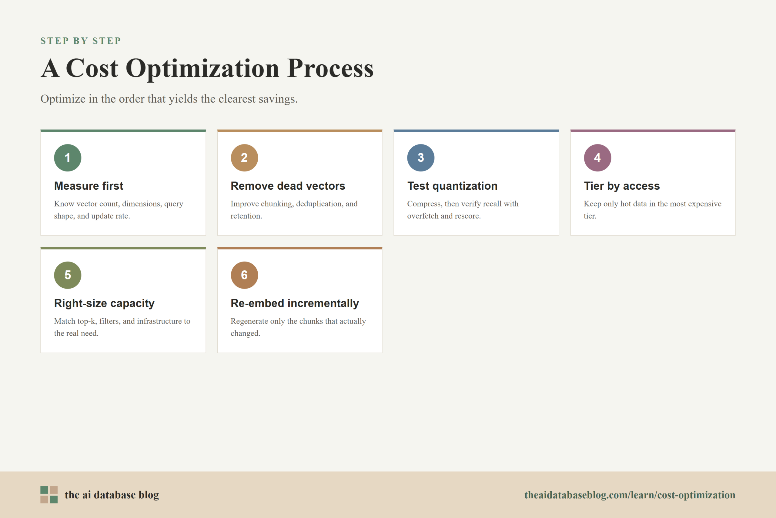
A strong cost optimization process begins with measurement. Teams should know how many vectors they store, how many dimensions those vectors have, how much memory the index consumes, how many queries run per day, how many candidates each query retrieves, how often documents are updated, and how often embeddings are regenerated. Without those numbers, cost discussions become guesswork.
After measurement, optimize in the order that usually produces the clearest savings. First, remove unnecessary vectors by improving chunking, deduplication, and retention. Second, test quantization or lower-precision storage against retrieval quality. Third, tier data so rarely used vectors do not occupy the most expensive tier. Fourth, right-size capacity and query parameters. Fifth, decide whether serverless or provisioned economics better match the workload. Sixth, make ingestion incremental so re-embedding does not erase the savings.
Evaluation should stay attached to every cost change. A cheaper system that retrieves worse context may increase downstream model usage, produce lower-quality answers, or require more user retries. The best optimization is the one that lowers total cost per successful retrieval, not just cost per stored vector or cost per query.
Cost optimization is most useful when it is connected to application outcomes. For a RAG assistant, that outcome may be answer accuracy and latency. For product search, it may be conversion or click quality. For recommendations, it may be engagement and diversity. The right metric keeps the team from treating infrastructure cost as separate from retrieval usefulness.
Common Mistakes That Increase Vector Search Costs
Many vector search cost problems come from decisions that were reasonable during experimentation but never revisited. A prototype may embed every tiny text fragment, use high-dimensional vectors, retrieve a large candidate set, run without compression, and store all data in one hot index. That can be acceptable while proving the concept, but it becomes expensive when the same pattern is scaled to production.
One common mistake is assuming that more vectors always means better retrieval. In practice, redundant chunks can add cost while making search noisier. Another mistake is treating full-precision vectors as the default forever, even after quantization could preserve quality at lower memory cost. A third mistake is re-embedding whole documents when only a small part changed.
Teams also overspend when they ignore query shape. Large top-k values, weak filters, and broad searches across unrelated data increase query work. If a system serves multiple tenants, products, or content types, careful partitioning and metadata design can reduce unnecessary search scope while improving relevance.
The final mistake is optimizing too late. It is easier to design chunking, versioning, tiering, and evaluation into the system early than to retrofit them after the index has grown large. Cost-aware design does not mean premature austerity; it means making future changes possible without rebuilding everything.
FAQs
1. What is the biggest cost driver in vector search?
The biggest cost driver is often memory, especially when large numbers of high-dimensional vectors and index structures need to stay available for low-latency search. Query volume, compute, replication, and ingestion work can also become major drivers depending on the workload.
2. Does quantization always reduce cost without hurting quality?
Quantization can reduce memory and storage cost, but it can also affect recall or ranking quality. The right approach is to test compressed search against a representative evaluation set and, when needed, use candidate overfetching and rescoring to recover quality.
3. When should vector data be moved to a warm or cold tier?
Vector data is a good candidate for a warm or cold tier when it is rarely queried, less time-sensitive, archived, or only needed for specific fallback searches. The decision should consider access frequency, business importance, freshness, and whether slower retrieval would harm the user experience.
4. Is serverless vector search cheaper than provisioned infrastructure?
Serverless can be cheaper for unpredictable, bursty, or early-stage workloads because it reduces idle capacity. Provisioned infrastructure can be cheaper for steady, high-utilization workloads where reserved capacity is used efficiently. The better choice depends on real traffic and query patterns.
5. How can teams reduce re-embedding cost?
Teams can reduce re-embedding cost by using incremental ingestion, storing chunk hashes, tracking embedding model versions, separating metadata updates from text changes, and re-embedding only changed chunks. For model upgrades, a staged backfill into a new index or namespace is often safer than a full immediate rebuild.
6. Can smaller embeddings lower vector search costs?
Yes. Smaller embeddings can reduce storage, memory, and distance-computation cost because each vector has fewer dimensions. The tradeoff is that smaller embeddings may or may not preserve retrieval quality for a specific dataset, so they should be tested against the application’s relevance metrics.
Takeaway
Cost optimization for vector search is most effective when teams treat memory, compute, query behavior, deployment model, and re-embedding as connected parts of the same retrieval system. Readers building AI databases, RAG applications, semantic search, or recommendation systems should focus first on measuring vector count, dimensionality, query shape, and ingestion work, then apply quantization, tiering, right-sizing, and incremental updates where they preserve retrieval quality. For a practical use case such as a support assistant, this means keeping active knowledge in a fast searchable tier, compressing or tiering older content, tuning top-k and filters, and re-embedding only the chunks that actually changed.