The right index for an AI database workload depends on what you are optimizing for: exactness, latency, memory use, update behavior, and filtered retrieval quality. Small datasets or highly selective filtered queries often work well with exact search because the candidate set is already manageable. HNSW is usually a strong default for low-latency, high-recall vector search when the dataset and graph fit comfortably in memory. IVF-style indexes become more attractive as datasets grow, top-k values increase, or memory efficiency matters. Quantized indexes reduce memory and storage cost, while disk-backed approaches are useful when the corpus is too large to keep fully in RAM.
This guide explains how to choose an index by reading the workload first instead of starting with a favorite algorithm. It covers the practical signals that matter most in AI database systems: dataset size, latency targets, memory budget, update frequency, and filtering needs. By the end, you should be able to narrow a workload to a reasonable index family, understand the tradeoffs behind that choice, and know what to test before putting the index into production.
Why Index Choice Matters in AI Databases
An index is a data structure that helps a database search faster than it could by scanning every vector or record. In an AI database, the index usually supports nearest neighbor search over embeddings, although it may also work alongside scalar indexes for metadata filters. The index determines how many vectors the system must inspect, how much memory the search path consumes, how much recall is lost through approximation, and how easily new records can be added or deleted.
The most important point is that there is no universally best index. A fast index for one workload can be a poor fit for another if the dataset size, query pattern, or filtering behavior changes. For example, a graph index can be excellent for finding a small number of close matches with low latency, but it may use more memory than a partitioned or quantized index. A compressed index can make a large corpus affordable, but it may need extra reranking to recover relevance. A disk-backed index can handle much larger corpora, but storage latency and I/O patterns become part of the performance equation.
This is why index selection should begin with the workload rather than the index name. Before choosing among exact search, HNSW, IVF, quantized variants, or disk-backed methods, define what the system must do under realistic traffic, data volume, and filtering conditions.
The Main Index Families to Understand
Most AI database index choices fall into a few broad families. Different systems use different names and implementation details, but the underlying tradeoffs are similar. Understanding these families makes it easier to reason about a workload without memorizing every database-specific option.
Exact or Flat Indexes
An exact, flat, or brute-force search compares the query vector against every vector in the candidate set. This gives the most reliable result because it does not approximate the nearest neighbors. It also avoids training and complex tuning. The cost is that query time grows with the number of candidates and the dimensionality of each vector.
Exact search is often better than people expect when the dataset is small, the filtered subset is tiny, the application runs only a few searches, or GPU acceleration is available. It is also useful as a baseline for evaluating approximate indexes because it shows what the best possible recall looks like for a given embedding model and distance metric.
HNSW and Other Graph-Based Indexes
HNSW, short for Hierarchical Navigable Small World, is a graph-based index. It connects vectors to nearby vectors, then searches by navigating through that graph from broad neighborhoods toward closer candidates. HNSW is widely used because it can deliver strong recall with low latency, especially for workloads that retrieve a modest number of results from an in-memory index.
The main tradeoff is memory. HNSW stores both vector data and graph connections, so it usually has meaningful per-vector overhead. Parameters such as graph degree and search breadth can improve recall, but they also increase memory use, build time, or query cost. HNSW also needs careful handling for deletes, updates, and heavy filtering, depending on the database implementation.
IVF and Partition-Based Indexes
IVF, or inverted file indexing, partitions vectors into clusters. At query time, the system searches only the clusters whose centroids are close to the query vector. This reduces the number of vectors examined, which can help with larger datasets and higher-throughput workloads.
IVF typically requires training so the system can learn useful clusters. It also needs tuning, commonly by choosing how many clusters exist and how many clusters are searched per query. Searching more clusters improves recall but increases latency. IVF-style indexes can be a good fit when the dataset is large, the top-k is relatively large, or memory efficiency is more important than squeezing out the lowest possible latency for small top-k queries.
Quantized Indexes
Quantization stores vectors in a smaller representation. Scalar quantization may reduce each dimension from a 32-bit float to a smaller numeric form, while product quantization splits vectors into parts and encodes those parts using compact codes. Quantization can make large indexes much cheaper to store and search, but it introduces approximation error because the stored representation is less precise than the original vector.
Many production systems compensate by retrieving more candidates than needed and reranking those candidates with higher-precision vectors. This approach can give a practical balance: the compressed index reduces memory and search cost, while reranking improves final result quality. Quantized indexes are most useful when the raw vectors are too large for the memory budget or when cost matters more than achieving the simplest high-recall setup.
Disk-Backed Indexes
Disk-backed vector indexes move some index data or vector data out of RAM and onto SSD-backed storage. DiskANN-style approaches are designed for large datasets where keeping the full corpus in memory is too expensive or impossible. They can make billion-scale retrieval more practical, but the workload must be designed around storage access patterns, I/O limits, and the extra latency that can appear when search needs to read from disk.
Disk-backed indexes are not automatically the best choice just because a dataset is large. If a workload has strict low-latency targets and enough RAM, an in-memory graph or partitioned index may still be better. Disk-backed methods become more compelling when memory is the limiting constraint and the system can tolerate the storage behavior required to serve large-scale retrieval.
Once these index families are clear, the next step is to map them to concrete workload signals. The same index family can behave very differently depending on dataset size, latency goals, memory pressure, write patterns, and metadata filters.
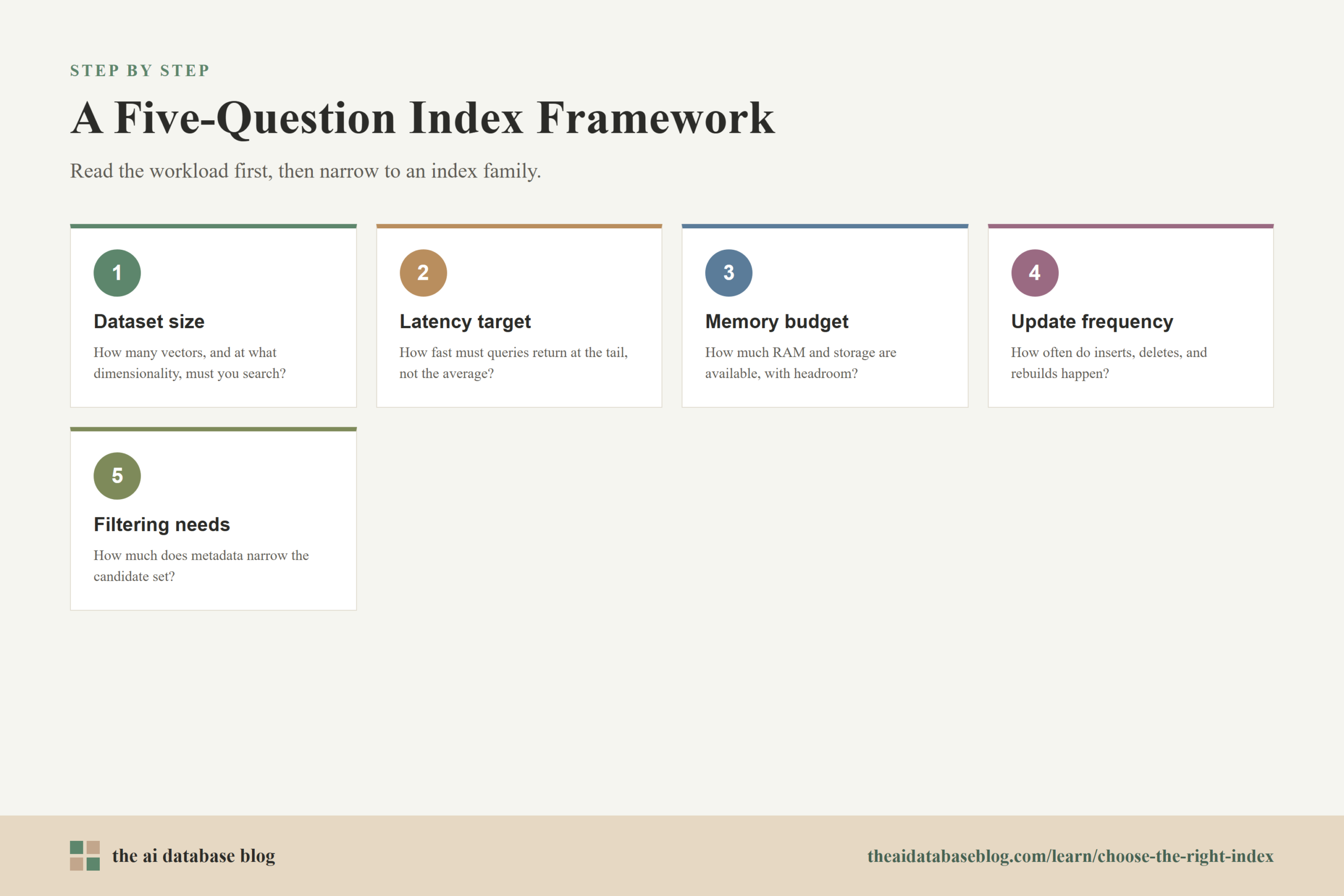
A Decision Framework for Choosing an Index
A good index decision starts with five questions. How many vectors will the system search? How fast must queries return? How much RAM and storage are available? How often does the data change? How much does filtering narrow the candidate set? Answering these questions in order helps prevent common mistakes, such as choosing a memory-heavy graph index for a corpus that cannot fit in RAM or choosing an approximate index for a workload where filters already reduce the search space to a few thousand records.
Start With Dataset Size
Dataset size is the first narrowing signal because it determines whether simple search is still practical. For thousands or low millions of vectors, exact search or HNSW may be enough, depending on latency requirements and hardware. For millions to hundreds of millions of vectors, approximate indexes usually become necessary because scanning every vector for every query becomes too expensive. For hundreds of millions to billions of vectors, partitioning, compression, sharding, disk-backed search, or some combination of those techniques becomes central to the design.
Dataset size should not be measured only by vector count. Vector dimensionality matters too. One million 384-dimensional vectors has a very different memory footprint from one million 3,072-dimensional vectors. The number of replicas, retained raw vectors for reranking, metadata storage, and index overhead all contribute to the actual resource requirement.
Match the Index to Latency Targets
Latency targets determine how much approximation the system can use and how aggressively the index must be tuned. If a user-facing search experience needs low double-digit millisecond responses, an in-memory HNSW-style index is often a good starting point when the dataset fits. If the workload can tolerate higher latency for better cost efficiency, IVF with careful probing, quantization with reranking, or disk-backed retrieval may be acceptable.
Latency should be measured at the percentile that matters for the product, not only as an average. A system with good median latency but poor tail latency may feel unreliable in production. Index parameters also change latency. Increasing HNSW search breadth or IVF probes can improve recall, but it makes each query do more work. Choosing an index is therefore also choosing the shape of the recall-latency curve you want to tune.
Use Memory Budget as a Hard Constraint
Memory budget often decides whether an ideal index is realistic. HNSW can be fast and accurate, but graph links add overhead on top of the vectors themselves. IVF-style indexes can be more memory efficient because they partition the space and may avoid some graph overhead. Quantization reduces the vector representation, which can lower RAM and storage cost dramatically, but it usually requires validation to ensure the compressed representation does not damage relevance.
A practical rule is to calculate the raw vector footprint first, then add index overhead and operational headroom. Raw vector storage is roughly the number of vectors multiplied by dimensions multiplied by bytes per dimension. A 32-bit floating point embedding uses four bytes per dimension. The real deployment also needs room for metadata, replicas, temporary query candidates, background indexing, and future growth. If the index only fits on paper but leaves no headroom, it is probably the wrong choice.
Account for Update Frequency
Update frequency changes the index decision because not all indexes handle inserts, deletes, and rebuilds equally well. Some graph indexes support incremental inserts well enough for many workloads, but deletes and compaction can still require careful management. IVF-style indexes depend on clustering, so a dataset whose distribution changes significantly may need retraining or rebuilding. Quantized indexes may also need retraining if the embedding distribution changes.
For mostly static corpora, such as archived documents or product catalogs updated in batches, heavier index build time may be acceptable. For streaming or frequently changing data, choose an index and database architecture that supports fresh inserts, predictable background indexing, and safe rebuilds. In many AI applications, it is useful to separate the source of truth from the search index so the index can be rebuilt when embeddings, chunking, or indexing strategy changes.
Treat Filtering as a First-Class Requirement
Filtering is one of the easiest ways to choose the wrong index if it is considered too late. AI database queries often combine vector similarity with metadata conditions such as tenant, language, category, access permission, date range, geography, or document type. The index must support not just vector similarity, but vector similarity after the relevant filters are applied.
There are three common patterns. Pre-filtering narrows the candidate set before or during vector search, which can improve result quality for selective filters but may increase traversal work. Post-filtering runs vector search first and applies filters afterward, which can be faster but may return too few qualifying results when filters are selective. Partitioning or partial indexing can be effective when filters are stable and commonly used, such as tenant-specific or category-specific retrieval.
Filtering can even make exact search the right answer. If a query filters a billion-row corpus down to a few thousand eligible records, brute-force search over the filtered subset may be simpler and more accurate than forcing an approximate global index to behave well under a highly selective predicate.
These five questions narrow the choice, but the final decision is easier when the signals are converted into practical rules. The next section turns the framework into concrete index recommendations for common workload shapes.
Practical Index Choices by Workload Pattern
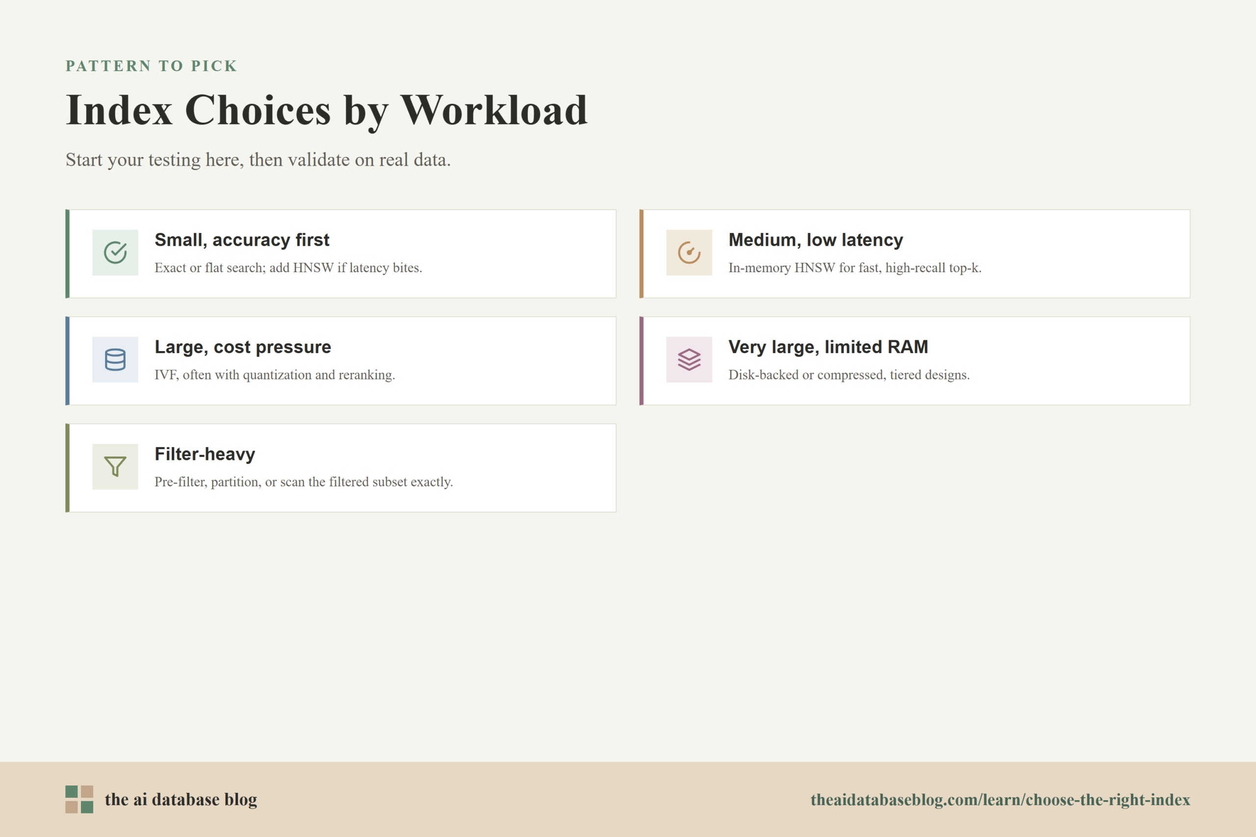
Most workloads are combinations of the same pressures: small or large data, tight or relaxed latency, abundant or limited memory, static or changing data, and simple or selective filters. The patterns below are not rigid rules, but they give a useful starting point for choosing what to test first.
Small Dataset With High Accuracy Needs
Use exact search or a simple flat index when the dataset is small enough that scanning candidates meets the latency target. This is especially sensible during early development, when the team is still evaluating chunking, embedding models, and relevance criteria. Exact search also makes it easier to measure whether an approximate index is losing important results.
If latency becomes a problem but the corpus still fits easily in memory, HNSW is a natural next step. It can reduce query time while preserving strong recall when tuned well.
Medium Dataset With Low-Latency Search
Use HNSW when the corpus fits in memory, the application needs fast top-k retrieval, and recall matters. This pattern is common in semantic search, RAG retrieval, recommendations, and similarity search over a manageable but growing corpus. The main tuning work is to balance graph construction, memory use, search breadth, and recall.
HNSW is not a free default. If the memory budget is tight, filters are highly selective, or updates are heavy, validate those conditions directly rather than relying only on unfiltered benchmark results.
Large Dataset With Throughput and Cost Pressure
Use IVF or IVF with quantization when the dataset is large enough that graph memory becomes expensive or when high throughput matters more than maximum per-query recall. IVF can reduce the search space by routing queries to relevant clusters, and quantization can reduce the cost of storing and comparing vectors.
This pattern requires more tuning than a simple flat or HNSW setup. You need representative training data, a sensible number of clusters, and query-time settings that balance recall and latency. If the index uses compression, test reranking with original or higher-precision vectors to recover result quality.
Very Large Dataset With Limited RAM
Use disk-backed search, compressed indexes, memory mapping, or a tiered design when the raw vectors and index cannot fit comfortably in memory. Disk-backed graph indexes can make much larger corpora searchable, while compressed IVF or graph variants can reduce memory pressure. The right choice depends on whether the workload is more constrained by RAM, storage I/O, recall, or latency.
For these workloads, capacity planning is part of index selection. Test with realistic concurrency, not only a single query. A design that works for isolated searches can fail under production traffic if SSD reads, cache misses, or reranking steps become bottlenecks.
High-Update Workload
Use an index strategy that supports freshness without constant full rebuilds. For append-heavy data, an index with incremental insertion support may be enough. For frequent deletes, corrections, and embedding changes, plan for compaction, segment merging, background rebuilds, or separate hot and cold indexes.
High-update workloads should also consider whether the embedding distribution changes over time. If a new embedding model or chunking strategy is introduced, the old index may no longer be representative. In that case, rebuildability is as important as query speed.
Filter-Heavy Workload
Use pre-filtering, partitioning, partial indexes, or exact search over filtered subsets when metadata filters are highly selective. A filter-heavy workload is not just a vector search problem. It is a combined vector and structured query problem, and the right design may depend as much on metadata indexing as on the vector index.
If the filter keeps most of the corpus, approximate vector search remains useful. If the filter keeps only a tiny fraction, post-filtering can miss relevant results because the best unfiltered neighbors may not satisfy the predicate. In those cases, the system needs a way to search within the filtered candidate set or expand the approximate scan until enough qualifying results are found.
After selecting a candidate index family, the work is not finished. The choice must be validated with the actual embeddings, filters, query distribution, and relevance requirements of the application.
How to Validate the Index Before Production
Index selection should be tested against realistic data, not only documentation examples or generic benchmarks. The same index can perform differently across embedding models, dimensions, data distributions, filter selectivity, and query types. A strong validation process compares candidate indexes under the conditions the application will actually face.
Start with an exact-search baseline. Use it to measure recall for each approximate index and each tuning setting. Then test latency at relevant percentiles, such as p50, p95, and p99. Include common filters, rare filters, high-concurrency traffic, batch ingestion, updates, deletes, and index rebuild behavior. If the workload uses RAG, evaluate downstream answer quality too, because a small retrieval recall difference can matter if the missing document contains the answer.
A useful validation checklist includes:
- Recall against an exact-search baseline for representative queries.
- Latency at median and tail percentiles under realistic concurrency.
- Memory consumption during search, ingestion, and index build.
- Behavior under selective and nonselective metadata filters.
- Freshness after inserts, updates, deletes, and compaction.
- Relevance quality after compression and reranking.
- Operational cost, including replicas, storage, and rebuild time.
This validation step often reveals that the best index is not the most sophisticated one. It is the simplest index that meets recall, latency, memory, filtering, and update requirements with enough operational headroom.
Common Mistakes When Choosing an Index
Many indexing problems come from choosing an algorithm before defining the workload. The most common mistake is treating HNSW as an automatic default because it performs well in many unfiltered nearest neighbor benchmarks. It is often a good choice, but memory overhead, filtering behavior, update handling, and build cost still matter.
Another mistake is optimizing only for average latency. AI retrieval systems often fail at the tail, especially when filters are selective, candidate expansion is large, or disk access is involved. A third mistake is compressing vectors without measuring relevance loss. Quantization can be very effective, but the quality impact depends on the embedding distribution and the reranking strategy.
Teams also underestimate how often indexes need to change. New embedding models, new metadata filters, new tenants, and new product requirements can all shift the best index choice. A good architecture makes indexes rebuildable and measurable rather than treating the first index choice as permanent.
FAQs
1. What is the best default index for vector search?
HNSW is often a strong default when the dataset fits in memory and the workload needs low-latency, high-recall top-k search. However, it is not always the best choice. Exact search may be better for small or heavily filtered datasets, IVF may be better for larger throughput-oriented workloads, and quantized or disk-backed indexes may be necessary when memory is limited.
2. When should I use exact search instead of an approximate index?
Use exact search when the candidate set is small enough to scan within the latency target, when you need a recall baseline, or when filters reduce the search space dramatically. Exact search is also useful during development because it removes index approximation from the relevance evaluation.
3. How does memory budget affect index selection?
Memory budget affects both whether an index can run and how much headroom the system has under load. HNSW typically needs memory for raw vectors and graph links. IVF can be more memory efficient, especially with compression. Quantization and disk-backed designs help when raw vectors and index overhead exceed the available RAM.
4. Why do filters make vector indexing harder?
Filters make vector indexing harder because the nearest unfiltered vectors may not be valid results after the metadata condition is applied. If the system searches first and filters afterward, it can miss relevant filtered results. If it filters during search, it may need to traverse more candidates, which can increase latency. This is why selective filters need explicit testing.
5. Are quantized indexes safe for RAG applications?
Quantized indexes can be safe for RAG applications when they are validated against the original vectors and paired with reranking when needed. The risk is that compression changes distance estimates enough to drop useful context. Test retrieval recall and final answer quality before relying on a compressed index in production.
6. How often should an index be rebuilt?
An index should be rebuilt when the data distribution, embedding model, chunking strategy, or workload pattern changes enough that the old structure no longer represents the search space well. Some systems also rebuild or compact indexes after many updates or deletes. The right cadence depends on freshness needs, index type, and operational cost.
Takeaway
Choosing the right index for an AI database workload is a practical systems decision, not a search for the single best algorithm. Dataset size tells you whether exact search is still feasible or whether approximate search is required. Latency targets shape how aggressively the index must prune candidates. Memory budget determines whether in-memory graph search, partitioned search, quantization, or disk-backed retrieval is realistic. Update frequency affects how easily the index can stay fresh, and filtering needs decide whether the system must search inside a narrowed candidate set. This guidance is most useful for teams building semantic search, recommendation, or RAG systems where retrieval quality and operational cost both matter. A good use case is a growing knowledge base that needs fast answers with tenant, permission, and document-type filters: the best index is the one that meets those filtered recall and latency targets with enough memory and rebuild headroom to keep working as the corpus grows.