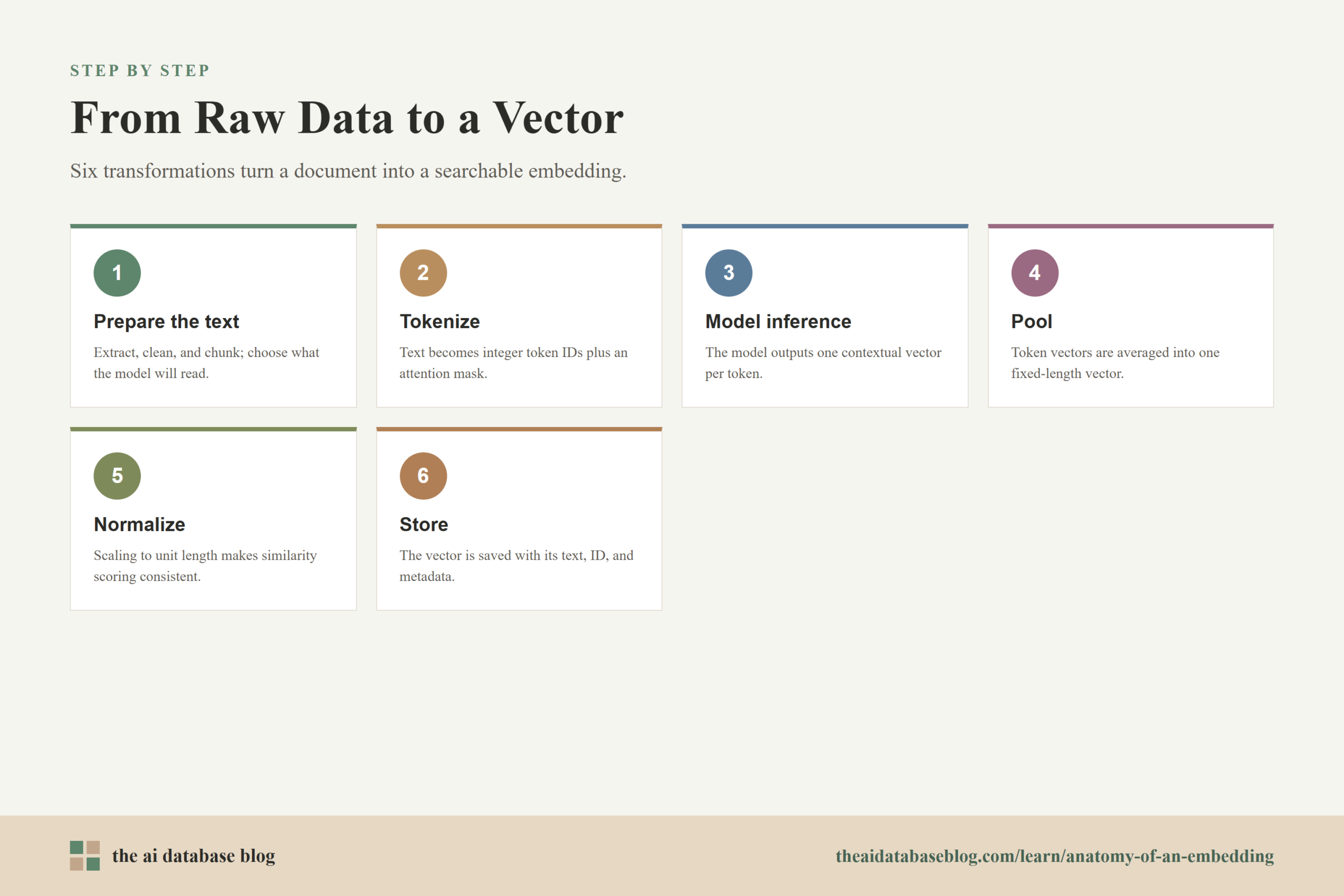
An embedding is a numerical representation of raw data that makes similarity search possible. For a text document, the path usually moves through a clear sequence: clean or chunk the raw document, tokenize the text into model-readable IDs, run those IDs through an embedding model, pool token-level outputs into one fixed-length vector, optionally normalize the vector, and store it with identifiers and metadata in a database. Each step changes the data shape, from human-readable text into arrays of numbers that can be indexed and compared.
This guide walks a single document through the embedding pipeline one stage at a time. By the end, you will understand what changes during tokenization, what the model actually receives, why pooling is needed, how normalization affects similarity search, and what an AI database stores when it saves an embedding for retrieval.
The Example Document Before Embedding
Before an embedding model can process a document, the system needs to decide what the document unit is. In retrieval systems, a “document” may be a full page, a paragraph, a passage, a support ticket, a table row, or a chunk extracted from a larger file. The important point is that the unit you embed becomes the unit the retrieval system can later return, score, filter, and cite.
For this walkthrough, imagine a short source document:
Document ID: policy_042
Title: Refund Policy
Text: Customers can request a refund within 30 days of purchase if the product is unopened.
At this stage, the data is still ordinary structured and unstructured content. A database or ingestion pipeline may already know the document ID, title, source, tenant, language, timestamp, and access rules. The embedding model, however, mainly needs the text string that will be converted into a vector.
A practical pipeline usually keeps two things separate but connected: the original content and the vector representation. The original content gives humans and language models something to read later. The vector gives the retrieval system a compact way to search by meaning.
Step 1: Prepare the Text That Will Be Embedded
The first transformation is not mathematical yet. It is a data preparation step that decides what text should be sent to the embedding model. This can include extracting text from a file, removing boilerplate, preserving useful headings, splitting long content into chunks, and attaching metadata that should not necessarily be embedded but should remain searchable or filterable.
For the example document, the text sent to the model might combine the title and body because the title adds useful context:
Refund Policy
Customers can request a refund within 30 days of purchase if the product is unopened.
This looks like a small change, but it matters. If the title is omitted, the vector may still represent the policy sentence well, but it may be less clearly connected to refund-related searches. If too much unrelated boilerplate is included, the embedding may become less focused. Embedding quality starts before the model sees the text.
Once the input text is chosen, the next question is how a model that only processes numbers can understand it. That is where tokenization begins.
Step 2: Tokenization Turns Text Into Model Inputs
Tokenization converts a text string into smaller units called tokens and then maps those tokens to integer IDs from the model’s vocabulary. Modern embedding models commonly use subword tokenization, which means unfamiliar words can be split into smaller pieces rather than treated as completely unknown. The tokenizer also often adds special tokens, creates an attention mask, and applies truncation or padding when needed.
A simplified tokenization result for the example might look like this:
Tokens:
["[CLS]", "refund", "policy", "customers", "can", "request", "a", "refund", "within", "30", "days", "of", "purchase", "if", "the", "product", "is", "unopened", ".", "[SEP]"]

Input IDs:
[101, 25416, 3343, 6304, 2064, 5227, 1037, 25416, 2306, 2382, 2420, 1997, 5309, 2065, 1996, 4031, 2003,  unopened_id, 1012, 102]

Attention mask:
[1, 1, 1, 1, 1, 1, 1, 1, 1, 1, 1, 1, 1, 1, 1, 1, 1, 1, 1, 1]
The exact tokens and IDs depend on the tokenizer used by the embedding model. The IDs above are illustrative, not a universal vocabulary. What matters is the structure: the text has become a sequence of integers, and the attention mask tells the model which positions contain real input rather than padding.
This is the first major shape change:
Before tokenization:
"Refund Policy Customers can request a refund within 30 days..."

After tokenization:
input_ids shape: [sequence_length]
attention_mask shape: [sequence_length]
For one document, the sequence length is the number of tokens after tokenization. In batch processing, many documents are processed together, so the shape becomes something like [batch_size, sequence_length]. Shorter inputs may be padded so each item in the batch has the same length.
Tokenization gives the model a numeric input, but these IDs are not yet the final embedding. They are lookup keys and control signals. The model still needs to transform them into contextual representations.
Step 3: Model Inference Creates Contextual Token Vectors
During model inference, the token IDs pass through the embedding model. The model first maps each token ID to an internal vector, adds positional information, and then applies layers of attention and feed-forward computation. The result is usually not one vector at first. It is a matrix of token vectors, where each token position has its own representation shaped by the surrounding words.
For a simplified example, imagine the model uses a hidden size of 768 dimensions and the input contains 20 tokens. The output may have this shape:
Token-level model output shape:
[20, 768]
That means the model produced 20 separate vectors, each with 768 numbers. The vector for “refund” near the beginning is not just a dictionary meaning of the word. It is a contextual vector influenced by “policy,” “customers,” “30 days,” “purchase,” and “unopened.” This is why transformer-based embeddings are more useful for retrieval than simple keyword counts: the representation reflects context, not just token presence.
A tiny illustrative slice of the token-level output might look like this:
Token: refund
Vector slice: [0.12, -0.04, 0.31, 0.08, ...]

Token: policy
Vector slice: [0.09, 0.17, -0.22, 0.05, ...]

Token: customers
Vector slice: [-0.03, 0.11, 0.28, -0.14, ...]
The full output contains far more numbers than shown here. Also, these numbers are not directly interpretable one by one. A single dimension rarely means “refundness” or “policy category” in a clean human-readable way. The meaning comes from the position of the whole vector in relation to other vectors.
At this point, the system has many token vectors, but most retrieval systems need one vector per stored passage. The next step compresses the token-level matrix into a single fixed-length document embedding.
Step 4: Pooling Converts Many Token Vectors Into One Embedding
Pooling is the step that turns variable-length token outputs into one fixed-length vector. A model may produce 20 token vectors for one short passage and 180 token vectors for a longer passage, but the database needs a consistent vector dimension for indexing. Pooling solves this by aggregating the token vectors into one representation.
Common pooling strategies include mean pooling, special-token pooling, max pooling, and model-specific learned pooling. Mean pooling is easy to understand: average the token vectors that correspond to real input tokens, usually using the attention mask so padding does not affect the result.
Token-level output:
[20, 768]

Pooling operation:
average the 20 token vectors across the sequence dimension

Document embedding:
[768]
In simplified form, mean pooling says: for each vector dimension, add the values from all real token positions and divide by the number of real tokens. If the first dimension across 20 tokens contains values such as 0.12, 0.09, -0.03, and so on, pooling averages those values into one number for the first dimension of the final embedding.
The result might look like this as a small slice:
Pooled embedding slice:
[0.034, 0.118, -0.062, 0.211, -0.009, ...]

Full vector shape:
[768]
Pooling is not just a technical convenience. It affects retrieval behavior. A pooling method that overemphasizes one token may produce different search results than one that averages across the full passage. This is why embedding models are usually trained and evaluated with a specific pooling approach, and why changing pooling after the fact can alter relevance.
Once pooling creates one vector, the system has something that looks like a usable embedding. But before it is stored, many pipelines apply normalization so similarity scoring behaves consistently.
Step 5: Normalization Makes Similarity Scoring More Consistent
Normalization adjusts a vector so its length has a chosen scale, often length 1. This is common when the retrieval system will use cosine similarity or dot product on normalized vectors. Normalization does not change the direction of the vector, but it changes its magnitude. In similarity search, that can make the score focus on angular similarity rather than vector length.
A simplified pooled vector might look like this before normalization:
Before normalization:
[0.034, 0.118, -0.062, 0.211, -0.009, ...]

Vector length:
3.42
After L2 normalization, each value is divided by the vector length:
After normalization:
[0.0099, 0.0345, -0.0181, 0.0617, -0.0026, ...]

Vector length:
1.00
The exact numbers here are illustrative, but the idea is accurate: the vector now lies on the unit sphere. If all stored vectors and query vectors are normalized, dot product and cosine similarity become closely aligned for ranking because both mainly measure whether vectors point in similar directions.
Normalization is not always mandatory. Some embedding models and retrieval systems expect normalized vectors; others preserve magnitude because it may carry useful information. The safest practical rule is to follow the embedding model’s recommended similarity metric and keep the same preprocessing for both stored documents and incoming queries.
Now the pipeline has a final vector that can be indexed. The last step is storage, where the AI database connects this numerical representation back to the original content and metadata.
Step 6: Storage Connects the Vector Back to the Document
An AI database or vector-capable database stores the embedding so it can be searched efficiently. The stored record usually includes a stable ID, the vector, the original text or a reference to it, metadata fields, and sometimes model information. This matters because retrieval is not only about nearest-neighbor math. Real applications also need filtering, permissions, versioning, updates, deletion, and traceability.
A simplified stored record might look like this:
{
  "id": "policy_042_chunk_001",
  "vector": [0.0099, 0.0345, -0.0181, 0.0617, -0.0026, "..."],
  "text": "Refund Policy. Customers can request a refund within 30 days of purchase if the product is unopened.",
  "metadata": {
    "document_id": "policy_042",
    "title": "Refund Policy",
    "source_type": "policy",
    "language": "en",
    "embedding_model": "example-text-embedding-model",
    "embedding_dimension": 768,
    "created_at": "2026-06-02"
  }
}
The vector field is what the database indexes for similarity search. The text field or document reference is what the application can return to a user or pass into a retrieval-augmented generation system. The metadata fields make it possible to filter results, group chunks by document, enforce access rules, or re-embed old content when a model changes.
Storage also introduces an important operational constraint: vectors produced by different embedding models should not be casually mixed in the same search space. A 768-dimensional vector from one model and a 768-dimensional vector from another model may have the same length but a different meaning. Even when dimensions match, the coordinate spaces may not be compatible.
With the document stored, the same pipeline can be applied to a user’s search query. Understanding that query path explains why the original document embedding is useful at retrieval time.
How the Stored Vector Is Used During Search
When a user asks a question such as “Can I get my money back after buying a product?”, the query is embedded through a similar process: tokenize the query, run model inference, pool the output, normalize if required, and compare the query vector with stored document vectors. The database then returns nearby vectors according to the selected similarity metric and any metadata filters.
The retrieval system is not matching the exact words “money back” to the exact word “refund” in a purely lexical way. Instead, it compares the query embedding to document embeddings in vector space. If the embedding model has learned that “money back” and “refund” are semantically related in this context, the refund policy chunk should rank near the query vector.
Query text:
"Can I get my money back after buying a product?"

Query vector:
[0.0121, 0.0298, -0.0214, 0.0583, ...]

Nearest stored vector:
policy_042_chunk_001
This is the core reason embeddings are useful in AI databases. They allow retrieval systems to search by semantic closeness, not only by exact word overlap. In practice, many systems combine vector search with keyword search, metadata filtering, reranking, or business rules to improve relevance and control.
Seeing the full path from raw document to retrieval result also makes it easier to understand common failure modes. If a result is poor, the problem may come from chunking, token truncation, the model choice, pooling behavior, normalization, metadata filters, or index configuration rather than from “the vector” as a single mysterious object.
What Changes at Each Stage
The embedding pipeline is easier to reason about when each stage is viewed as a data transformation. The raw document begins as text and metadata. Tokenization turns the text into IDs. Model inference turns IDs into contextual token vectors. Pooling turns many token vectors into one fixed-length vector. Normalization adjusts the vector length. Storage places the vector, text, and metadata into a searchable system.
Raw document:
text + metadata

Prepared input:
selected text string

Tokenized input:
input_ids + attention_mask

Model output:
token vectors, shape [sequence_length, hidden_size]

Pooled embedding:
one vector, shape [hidden_size]

Normalized embedding:
one vector with controlled length

Stored record:
id + vector + text/reference + metadata
This sequence is useful because it separates conceptual meaning from implementation details. Different models may use different tokenizers, dimensions, pooling strategies, and recommended similarity metrics. Different databases may store text and metadata differently. But the broad transformation pattern remains stable across most text embedding pipelines used for AI retrieval.
Once the stages are clear, the practical design questions become more concrete. You can ask whether the input text is well formed, whether the chunk size fits the model, whether the chosen vector dimension is appropriate, whether normalization matches the similarity metric, and whether the stored metadata supports the retrieval workflow.
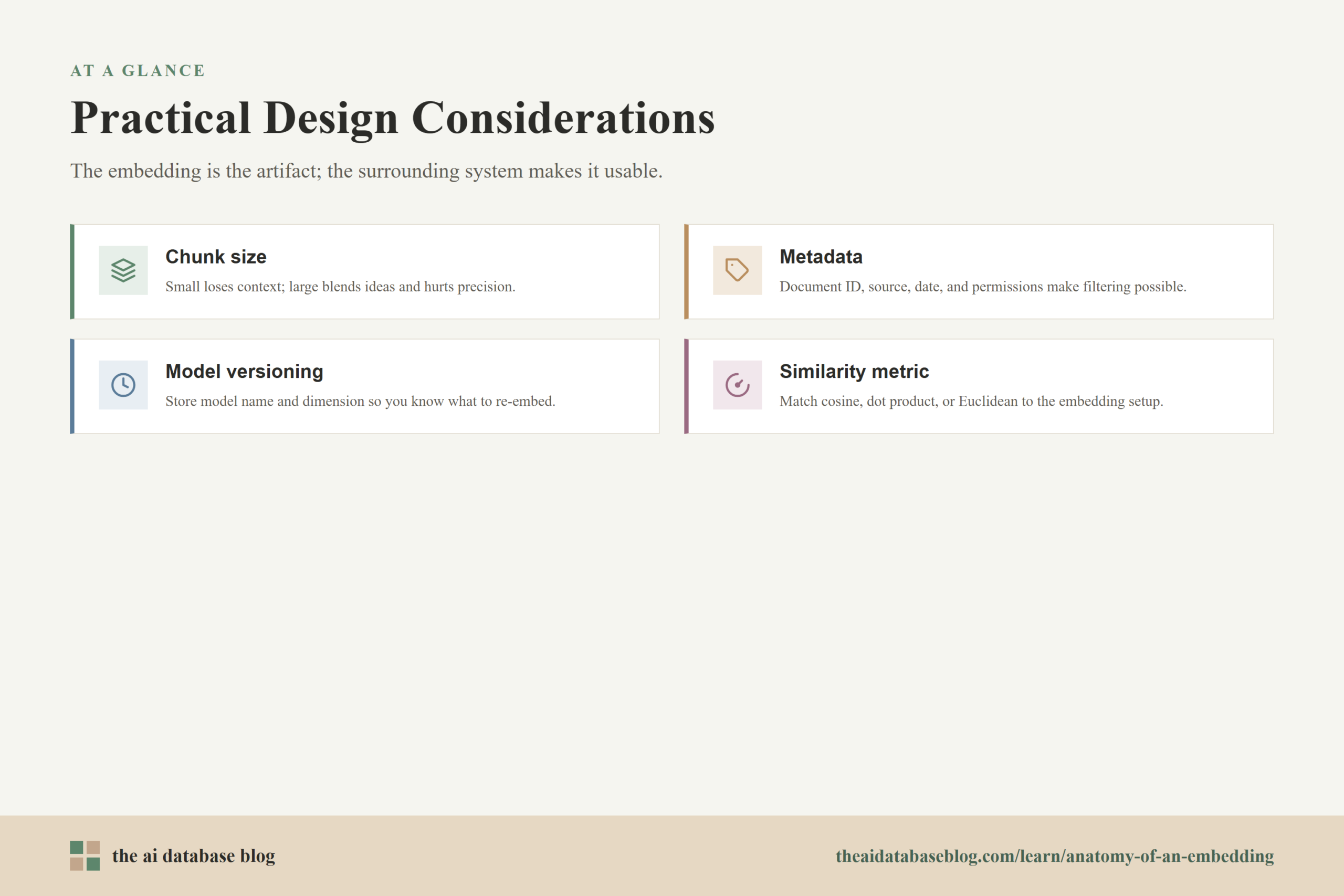
Practical Design Considerations for AI Databases
An embedding pipeline is not only a model call. It is part of a data system. The decisions made around chunking, metadata, versioning, and storage shape how useful the vectors are in production. A technically valid embedding can still perform poorly if the document unit is too broad, the source text loses important context, or the database cannot filter results in the way the application needs.
Chunk Size Affects Meaning and Retrieval Granularity
If a chunk is too small, it may not contain enough context for a meaningful embedding. If it is too large, unrelated ideas may be blended into one vector, and the returned result may be less precise. Good chunking usually aims for passages that are complete enough to answer a question but narrow enough to retrieve a specific idea.
Metadata Makes Vectors Operational
Metadata gives retrieval systems control beyond similarity scoring. Fields such as document ID, source, date, language, tenant, user permissions, and content type can help the database filter candidates before or during vector search. Without metadata, every query risks searching a space that is broader than the application actually intends.
Model Versioning Prevents Mixed Vector Spaces
When an embedding model changes, the meaning of the vector space may change too. Storing the embedding model name, version, dimension, and creation time helps teams know which records need re-embedding. This is especially important when old and new embeddings coexist during migration.
Similarity Metric Should Match the Embedding Setup
Cosine similarity, dot product, and Euclidean distance are not interchangeable in every setup. A normalized vector paired with dot product can behave differently from an unnormalized vector paired with the same metric. The best choice depends on how the model was trained and what the database expects.
These design choices are where embedding pipelines become AI database architecture. The vector is the visible artifact, but the surrounding system determines whether that vector can be trusted, updated, filtered, and used in a real application.
FAQs
1. Is an embedding the same thing as a token vector?
No. A token vector usually refers to a representation for one token position inside the model. A document embedding is usually a pooled representation for the whole input passage. Token vectors are intermediate outputs, while the final embedding is the vector commonly stored for retrieval.
2. Why does the tokenizer create IDs instead of sending words directly to the model?
Models process numbers, not raw characters or words. The tokenizer maps text into integer IDs from a fixed vocabulary so the model can look up and transform those IDs into internal numerical representations. The tokenizer also handles special tokens, masks, padding, and truncation.
3. Why is pooling necessary?
Pooling is necessary because documents have different numbers of tokens, but a vector database typically needs one fixed-length vector for each stored item. Pooling turns a variable-length matrix of token vectors into a single vector with a consistent dimension.
4. Does normalization improve every embedding search system?
Not always. Normalization is useful when the model and similarity metric are designed around vector direction, such as cosine-style retrieval. Some systems may intentionally preserve vector magnitude. The important rule is to use the same normalization and metric strategy for both stored documents and query embeddings.
5. What does a vector database store besides the vector?
It often stores an ID, the vector, the original text or a pointer to it, and metadata such as source, document ID, language, permissions, model version, and timestamps. The exact storage design depends on the application, but metadata is essential for filtering, governance, and updates.
6. Can two embedding models share the same vector index?
Usually they should not be mixed unless the system is designed for that. Even if two models produce vectors with the same number of dimensions, their vector spaces may encode meaning differently. In most retrieval systems, embeddings from different models are separated or carefully migrated.
Takeaway
An embedding is the final result of a series of transformations: raw text is prepared, tokenized into model inputs, transformed into contextual token vectors, pooled into one fixed-length representation, normalized when appropriate, and stored with text and metadata in an AI database. This understanding is useful for developers, data engineers, and product teams building semantic search, retrieval-augmented generation, support automation, or knowledge retrieval systems because it shows where relevance, performance, and maintainability are actually shaped.