HNSW, short for Hierarchical Navigable Small World, is a graph-based indexing algorithm used to make high-dimensional vector search fast enough for practical AI applications. Instead of comparing a query vector with every stored vector, HNSW organizes vectors into a layered proximity graph, starts search from sparse upper layers, and uses greedy traversal to move toward increasingly similar neighbors. Its main appeal is that it can deliver high-recall approximate nearest neighbor search with sublinear, often near-logarithmic search behavior, but that speed comes with meaningful memory cost because the index stores both vectors and graph connections.
This guide explains how HNSW works from the inside out. It covers the hierarchical navigable small world graph, the layered structure that makes search efficient, how greedy traversal moves through the graph, why people describe HNSW search as logarithmic in practice, where the algorithm is strongest, and why memory planning matters when using it in AI databases and retrieval systems.
What HNSW Is Solving
AI databases often need to search through large collections of embeddings, which are numerical representations of text, images, audio, code, or other data. The basic task is nearest neighbor search: given a query vector, find the stored vectors that are closest according to a distance or similarity measure such as cosine similarity, dot product, or Euclidean distance. A direct exact search is simple to understand, but it becomes expensive as the collection grows because the database must compare the query against many or all vectors.
HNSW solves this by building an approximate nearest neighbor index. The word approximate matters: HNSW is designed to find very good nearest neighbor candidates quickly, not to prove that it has found the exact best match in every case. For many AI applications, including retrieval-augmented generation, semantic search, recommendations, and similarity lookup, this tradeoff is useful because a small loss in recall can produce a large gain in latency.
The key idea is that vectors can be organized as a graph where each vector is connected to nearby vectors. Once the graph is built, search becomes a navigation problem. Instead of scanning the whole dataset, the algorithm moves from node to node, choosing neighbors that appear closer to the query until it reaches a region of the graph where the best candidates are likely to live.
Understanding HNSW starts with understanding why the graph is called a small world graph. The phrase describes a network where most points are locally clustered, yet the graph still provides short paths across distant regions. That combination of local detail and long-range reach is what allows HNSW to move quickly through a large vector space.
The Hierarchical Navigable Small World Graph
An HNSW index is built from a navigable small world graph. Each stored vector becomes a node, and each node keeps links to a limited number of nearby nodes. These links create a proximity graph: nodes that are close in vector space tend to be connected, so walking through the graph tends to move search toward more relevant areas.
The graph is navigable because a simple local rule can usually make progress. At each step, the algorithm looks at the neighbors of the current node and moves to a neighbor that is closer to the query. This is not the same as knowing the global nearest neighbor. It is a local decision that works well because the graph is structured so that local movement tends to lead toward better regions.
The small world property adds another important ingredient. A graph that only connects each node to very close neighbors can become slow to traverse because the search may have to take many small steps. A graph with some longer-range connections can cross the space more quickly. HNSW uses hierarchy to create those long-range navigation paths in a controlled way.
This is the first major difference between HNSW and a plain nearest-neighbor graph. HNSW does not rely on one flat graph alone. It builds several graph layers, where upper layers are sparse and lower layers are dense. The sparse layers help search move quickly across broad regions, while the dense bottom layer supports careful local search.
Once the graph idea is clear, the next question is how HNSW decides which connections belong in which part of the index. That is where the layered structure becomes central.
How The Layered Structure Works
HNSW organizes nodes into multiple layers. Every vector appears in the bottom layer, often called layer 0. A smaller subset of vectors appears in the layer above it, an even smaller subset appears above that, and so on until the top layer contains only a few entry points. This layout resembles a tower-like structure: most nodes exist only at the base, while a few nodes extend upward into higher layers.
When a new vector is inserted, HNSW assigns it a maximum layer using a probability-based process. Most vectors receive only a low layer. A smaller number receive higher layers. This creates a natural hierarchy without manually clustering the dataset into fixed partitions. The result is a stack of related graphs, each giving the search process a different level of detail.
The upper layers act like express lanes. Because they contain fewer nodes, the search can make large jumps across the vector space with relatively few comparisons. These layers do not need to contain every fine-grained local relationship. Their job is to help the algorithm find a promising region quickly.
The bottom layer is where most of the precision comes from. Since every vector is present there, HNSW can expand the candidate set around the region discovered from the upper layers and look for the best approximate neighbors. This final layer is denser and more expensive to search, but the earlier layers reduce how much of it must be explored.
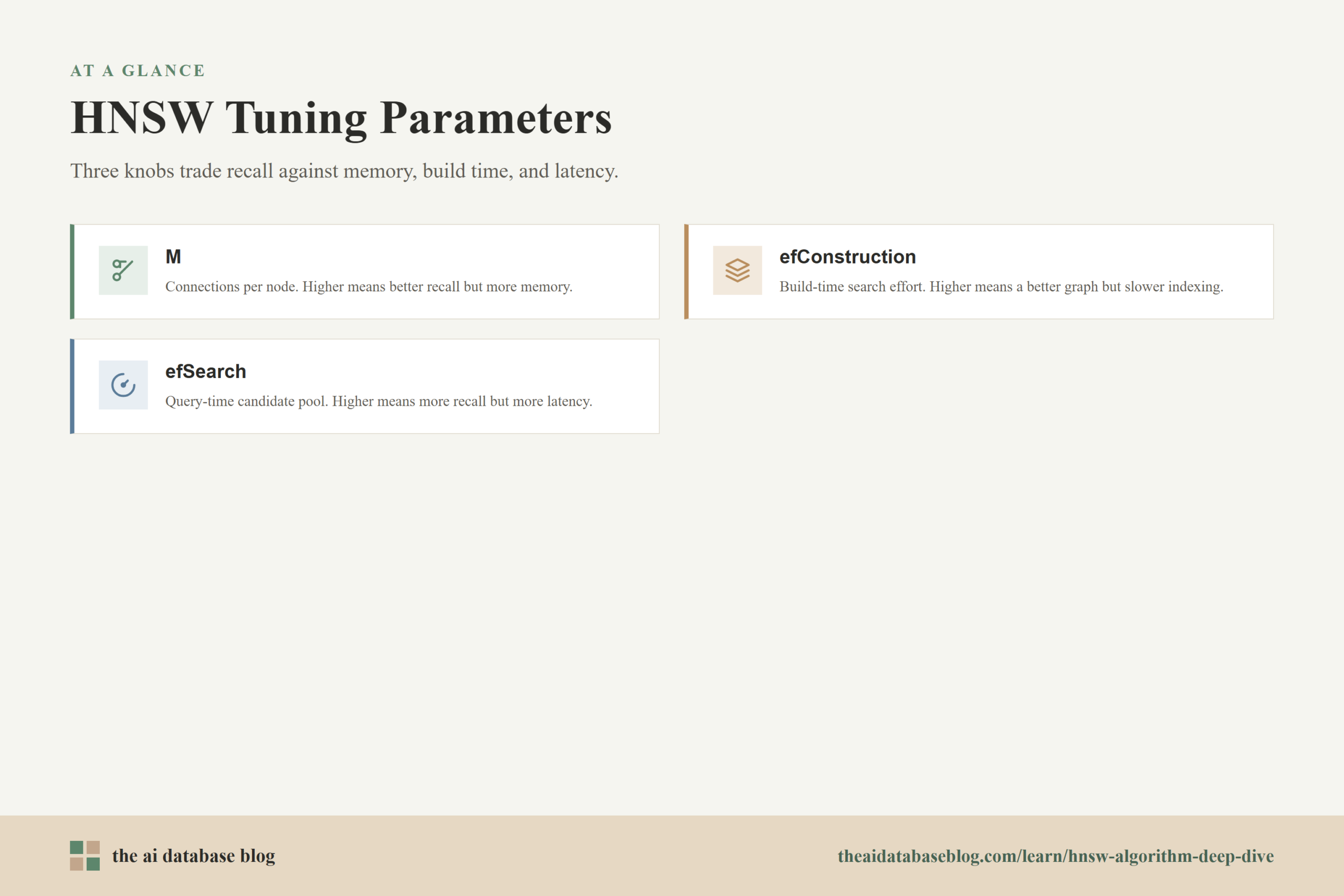
Several index parameters influence this structure. A common parameter, often called M, controls how many graph connections each node can keep. Larger values create a denser graph with better navigation and usually better recall, but they also increase memory use. Another parameter, often called efConstruction, controls how broadly HNSW searches while building the index. Higher values can improve graph quality, but they make index construction slower.
The layers explain the shape of the index, but they do not fully explain the search behavior. To see why HNSW is fast, it helps to follow what happens when a query enters the index.
Greedy Traversal During Search
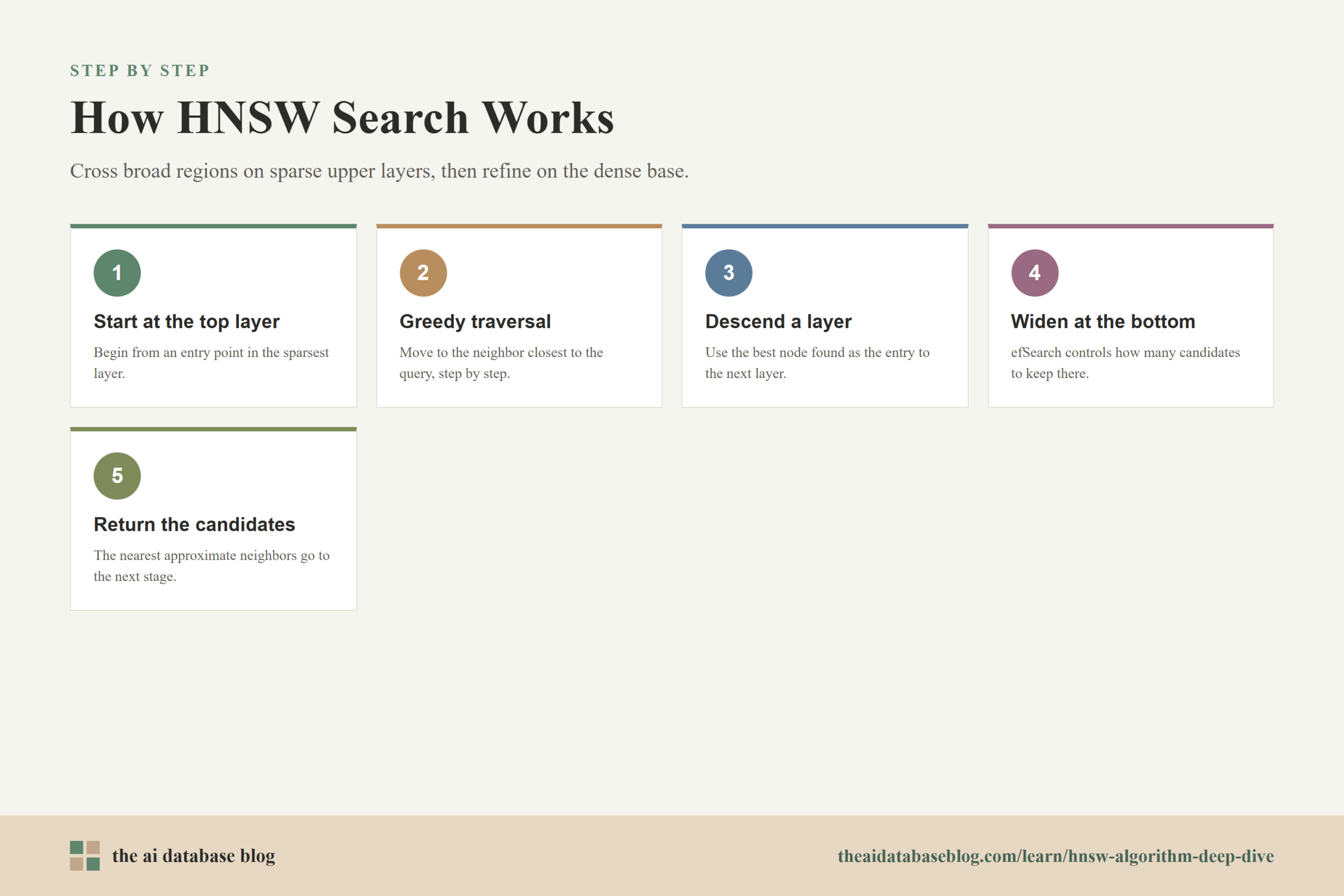
HNSW search begins at an entry point in the highest available layer. From there, the algorithm compares the query vector with neighboring nodes and moves to a neighbor if that neighbor is closer to the query than the current node. It repeats this process until no neighbor in that layer improves the distance. At that point, the best node found in the current layer becomes the entry point for the next layer down.
This top-down movement is greedy because the algorithm keeps choosing locally better positions. It does not explore every possible path through the graph at the upper layers. Instead, it uses each sparse layer to get closer to the query region, then descends into a more detailed layer and continues from the best position found so far.
At the bottom layer, HNSW usually performs a wider search rather than a single greedy walk. A query-time parameter, often called ef or efSearch, controls how many candidate nodes the algorithm keeps while exploring the bottom graph. A larger efSearch means the algorithm considers more possibilities, which can improve recall, but it also increases distance calculations and latency.
A simple way to picture the process is to imagine looking for a house in an unfamiliar city. The top layer gets you to the right part of the city. The middle layers get you to the right neighborhood. The bottom layer searches the nearby streets. HNSW is effective because it avoids checking every street in every neighborhood.
This traversal pattern also explains why HNSW performs well for many retrieval workloads. It spends most of its effort near promising candidates instead of spreading work evenly across the entire dataset. The next question is why this can lead to search costs that are often described as logarithmic.
Why HNSW Can Achieve Logarithmic Search Cost
HNSW is often described as having logarithmic or near-logarithmic average search behavior because the hierarchy shrinks the search problem as it moves downward. The upper layers contain only a small fraction of the total nodes, so the algorithm can use them to cross long distances quickly. Each descent brings the search closer to the dense base layer, but it starts that layer from a much better position than a random entry point would provide.
The comparison to logarithmic search should be understood carefully. HNSW does not make every query cost exactly proportional to the logarithm of the dataset size. Real performance depends on data distribution, dimensionality, graph quality, parameter choices, hardware, distance metric, and filtering behavior. However, the navigable small world structure is designed so that the number of steps needed to reach a useful region grows much more slowly than a full scan.
The hierarchy is what makes that possible. If a dataset doubles in size, HNSW does not simply double the work for every query in the way a brute-force scan might. More nodes may appear in the graph, but the upper layers still provide short routes through the space. Query cost is shaped by the number of graph hops and candidate expansions, not by a mandatory comparison against every vector.
In practical AI database use, this is why HNSW can support low-latency semantic search over large embedding collections. The exact latency still needs to be measured on the real workload, especially when metadata filters, hybrid ranking, or frequent updates are involved. Still, the algorithm’s structure gives it a strong scaling profile for many high-dimensional nearest neighbor search problems.
Search cost is only one side of the tradeoff. The reason HNSW became popular is not just that it is fast, but that it offers a practical balance of speed, recall, and operational simplicity for many AI systems.
Strengths Of HNSW
HNSW has become one of the most widely used vector indexing approaches because it works well across many common embedding search workloads. Its strengths come from the fact that it is graph-based, adaptive during search, and tunable through a small number of important parameters. For developers building AI database features, this makes HNSW easier to reason about than many more specialized indexing methods.
High Recall At Low Latency
The main strength of HNSW is that it can return high-quality approximate nearest neighbors without scanning the full vector collection. For retrieval systems, this is often the most important requirement. A search system needs to find relevant candidates quickly enough to support interactive use, while still returning results that are close enough to the true nearest neighbors to be useful.
Good Fit For High-Dimensional Embeddings
Many AI applications store embeddings with hundreds or thousands of dimensions. Traditional tree-based indexes often struggle as dimensionality rises because distance relationships become harder to partition cleanly. HNSW handles high-dimensional spaces well because it uses graph navigation rather than relying on rigid axis-aligned splits or fixed spatial partitions.
Tunable Accuracy And Speed
HNSW gives system designers practical control over the search tradeoff. Increasing efSearch generally improves recall because the algorithm explores more candidates, while decreasing it can reduce latency. Increasing M can improve graph connectivity and recall, while decreasing it saves memory. These controls make HNSW useful in systems where search behavior must be tuned to a latency budget.
Strong Query-Time Behavior For Read-Heavy Workloads
HNSW is especially attractive when the index is queried often and updated less frequently. Once the graph is built, searches can be very fast. That makes it a strong fit for semantic search, document retrieval, recommendation candidate generation, code search, image similarity search, and retrieval-augmented generation pipelines where the vector collection is large but not constantly rebuilt from scratch.
These strengths explain why HNSW is common in AI databases, but they should not hide the operational costs. The same graph structure that makes HNSW fast also consumes memory, and that memory cost can become the deciding factor at scale.
Memory Cost And Operational Tradeoffs
HNSW is usually memory-intensive because an index stores more than the raw vectors. It also stores graph connections, layer information, neighbor lists, and other index metadata. Each node must keep links to other nodes, and higher values of M increase the number of stored connections. As collections grow into millions or billions of vectors, these additional graph structures can become a major part of infrastructure planning.
The first memory component is the vector data itself. For example, high-dimensional float vectors can already require substantial storage before any index is added. The second component is the HNSW graph. The graph adds neighbor references for each node, and because the bottom layer contains every vector, the base graph is usually the largest part of the HNSW structure.
Memory cost is closely tied to performance. HNSW benefits from fast random access because traversal jumps between graph nodes and reads neighbor lists. If the index fits in memory, search can remain fast. If the system must constantly fetch graph data from slower storage, latency can become less predictable. This is why many production designs estimate vector memory and index memory together rather than treating the index as a small add-on.
There are also update tradeoffs. Insertions require the algorithm to search the existing graph, choose neighbors, and update connections. Deletes can be more complicated than simple removal because graph quality may suffer if many nodes are removed or marked inactive. Some systems use tombstones, background cleanup, compaction, or rebuild strategies to keep the graph healthy over time.
Filtering can add another practical wrinkle. If a query includes strict metadata filters, the nearest nodes in the graph may not be valid results. Depending on the system design, this can reduce recall or require broader exploration. In AI database applications, HNSW is often paired with metadata filtering, hybrid search, reranking, or partitioning strategies, so the real behavior should be tested with realistic queries rather than only with clean benchmark vectors.
Because memory and update behavior matter so much, HNSW works best when teams tune it deliberately. The next section explains how to think about those tuning choices without turning every deployment into a parameter guessing exercise.
How To Tune HNSW In Practice
Practical HNSW tuning starts with the workload goal. If the application needs very high recall, the index may need a larger M, a larger efConstruction during build, and a larger efSearch during query. If the application needs very low latency or must fit into a strict memory budget, those values may need to be lower. The right settings depend on the dataset, embedding model, query patterns, and acceptable recall-latency tradeoff.
M is one of the most important memory-related choices. A larger M gives each node more neighbors, which can make the graph easier to navigate and improve recall. The cost is that the graph stores more edges, increasing memory use. M also influences construction time because the algorithm has more candidate relationships to evaluate and maintain.
efConstruction controls how much effort HNSW spends while building the graph. Higher values usually create a better-connected index because the builder considers more candidates before choosing links. This can improve later search quality, but it increases indexing time. For relatively static collections, spending more time at build time can be worthwhile if it improves query performance later.
efSearch controls query-time exploration. Raising efSearch is often the easiest way to improve recall after an index already exists, because it tells the search process to keep a larger candidate pool. The tradeoff is higher latency because more candidates require more distance calculations. Many systems tune efSearch differently for different use cases, such as faster preview search versus deeper retrieval for high-value queries.
The safest tuning process is empirical. Start with a representative sample of vectors and real or realistic queries. Measure recall against an exact search baseline on a manageable subset. Then test latency, memory use, and result quality as M, efConstruction, and efSearch change. This helps reveal whether the application is recall-limited, latency-limited, memory-limited, or affected by filtering and reranking behavior.
Once these parameters are understood, HNSW becomes easier to place within a larger AI database architecture. It is not the whole retrieval system, but it is often the part that determines how quickly candidate vectors can be found.
Where HNSW Fits In AI Database Architecture
In an AI database, HNSW is typically the vector index used to retrieve candidate records from an embedding collection. The database stores the vector, the original or associated object, and metadata such as document IDs, timestamps, categories, access permissions, or source fields. HNSW helps find nearby vectors, while the rest of the database handles filtering, persistence, updates, ranking, and application-facing query behavior.
For retrieval-augmented generation, HNSW often sits near the beginning of the retrieval pipeline. A user query is converted into an embedding, the HNSW index retrieves semantically similar chunks or records, and those candidates may then be filtered, reranked, deduplicated, or assembled into context for a language model. The quality of the initial HNSW retrieval affects what information is available to every later stage.
For recommendation and similarity systems, HNSW can retrieve candidate items that are close to a user profile, product vector, image vector, or content vector. The final ranking may include business rules, freshness, popularity, permissions, or personalization signals. In these systems, HNSW is usually responsible for fast candidate generation rather than final ranking by itself.
The important architectural point is that HNSW is a retrieval primitive, not a complete relevance strategy. It finds nearby vectors efficiently, but application quality still depends on embedding quality, chunking strategy, metadata design, filter behavior, reranking, evaluation, and monitoring. A well-built HNSW index can make a system fast, but it cannot compensate for poor data modeling or weak relevance evaluation.
That broader view helps explain both the value and the limits of the algorithm. HNSW is powerful because it gives AI databases a fast way to navigate high-dimensional similarity space, but it should be evaluated as part of the complete retrieval workflow.
FAQs
1. What does HNSW stand for?
HNSW stands for Hierarchical Navigable Small World. The name describes the structure of the index: it is hierarchical because it uses multiple graph layers, navigable because search moves through connected nodes, and small world because the graph is designed to provide short paths between regions of the vector space.
2. Is HNSW exact or approximate?
HNSW is an approximate nearest neighbor algorithm. It is designed to return very close matches quickly, but it does not always guarantee the exact nearest neighbors. In many AI database workloads, this tradeoff is acceptable because the speed improvement is large and the returned candidates are usually relevant enough for downstream ranking or retrieval.
3. Why does HNSW use layers?
HNSW uses layers to make search efficient at different levels of detail. Sparse upper layers help the algorithm move quickly across broad regions of the graph, while the dense bottom layer contains all vectors and supports more careful local search. This hierarchy reduces the need to explore the full graph from scratch for every query.
4. What is greedy traversal in HNSW?
Greedy traversal means the search process repeatedly moves from the current node to a neighboring node that is closer to the query. In upper layers, this local decision helps the algorithm quickly approach a promising region. At the bottom layer, HNSW usually expands the search more broadly by keeping a candidate pool controlled by efSearch.
5. Why is HNSW often described as logarithmic?
HNSW is often described as logarithmic because its layered small world structure lets search reach useful regions through a small number of graph hops compared with scanning every vector. This is best understood as an average-case scaling property rather than a fixed guarantee. Actual cost depends on the dataset, parameters, hardware, filters, and query distribution.
6. What is the biggest downside of HNSW?
The biggest downside is memory cost. HNSW stores graph links in addition to the vectors themselves, and those links can require substantial memory at large scale. Higher-connectivity settings can improve recall, but they also increase memory use and build time. Teams using HNSW should plan memory, latency, and recall together.
Takeaway
HNSW is a practical and widely used algorithm for fast vector search because it turns nearest neighbor lookup into navigation through a layered graph. The upper layers help search move quickly toward the right region, greedy traversal guides the query through progressively closer nodes, and the bottom layer performs the detailed candidate search that supports high recall. This guide is most useful for engineers, architects, and technical readers designing AI database systems, especially for use cases such as semantic search, retrieval-augmented generation, recommendations, and similarity lookup. The main lesson is that HNSW offers strong search performance, but its memory cost, tuning parameters, filtering behavior, and update patterns must be planned carefully for production systems.