Approximate nearest neighbour search, often shortened to ANN search, is the method AI databases use to find highly similar vectors quickly without checking every vector exactly. It exists because exact nearest neighbour search becomes too slow and expensive as embedding collections grow into millions, hundreds of millions, or billions of records. ANN search trades a small amount of certainty for much lower latency, usually measured through recall: the share of true nearest results that the system successfully returns. The main algorithm families include graph-based indexes, inverted file indexes, quantization and compression methods, hashing methods, tree-based methods, and disk-aware or hybrid approaches that combine several ideas.
This guide explains why exact vector search becomes difficult at scale, what ANN search gives up in exchange for speed, how recall helps teams reason about quality, and how the major algorithm families fit together. By the end, you should be able to read an algorithm article, database configuration page, or vector search benchmark with a clearer sense of what is being optimized and what tradeoffs may matter for an AI application.
What Nearest Neighbour Search Means In AI Databases
Nearest neighbour search is the task of finding the stored items that are closest to a query item according to a chosen distance or similarity function. In an AI database, the stored items are usually embeddings: numerical vectors that represent text, images, audio, products, users, events, or other objects. A query is embedded into the same vector space, and the database looks for the vectors that are closest to it.
The word “nearest” does not mean physically close. It means close in the mathematical space created by the embedding model. If two paragraphs discuss similar ideas, their embeddings may sit near each other even if they use different words. If two images contain similar visual content, their image embeddings may be near each other even if their filenames or metadata have nothing in common.
AI databases use this operation for semantic search, recommendation, duplicate detection, clustering, retrieval-augmented generation, and many other workflows where exact keyword matching is not enough. A retrieval system might ask, “Which policy documents are closest to this user question?” A product search system might ask, “Which catalog items are closest to this description and match these filters?” A support assistant might ask, “Which previous tickets resemble this new issue?”
At small scale, nearest neighbour search can be simple. The system can compare the query vector with every stored vector, calculate each distance, sort the results, and return the closest matches. That approach is called exact search or brute-force search. It is easy to understand and gives the correct nearest neighbours according to the chosen metric, but it becomes difficult to sustain as the collection grows.
Once the basic task is clear, the next question is why an exact answer becomes so expensive. The answer is not only that there are many vectors. It is also that each vector may have hundreds or thousands of dimensions, each query may need to return results in milliseconds, and modern AI systems often run many searches at once.
Why Exact Search Does Not Scale
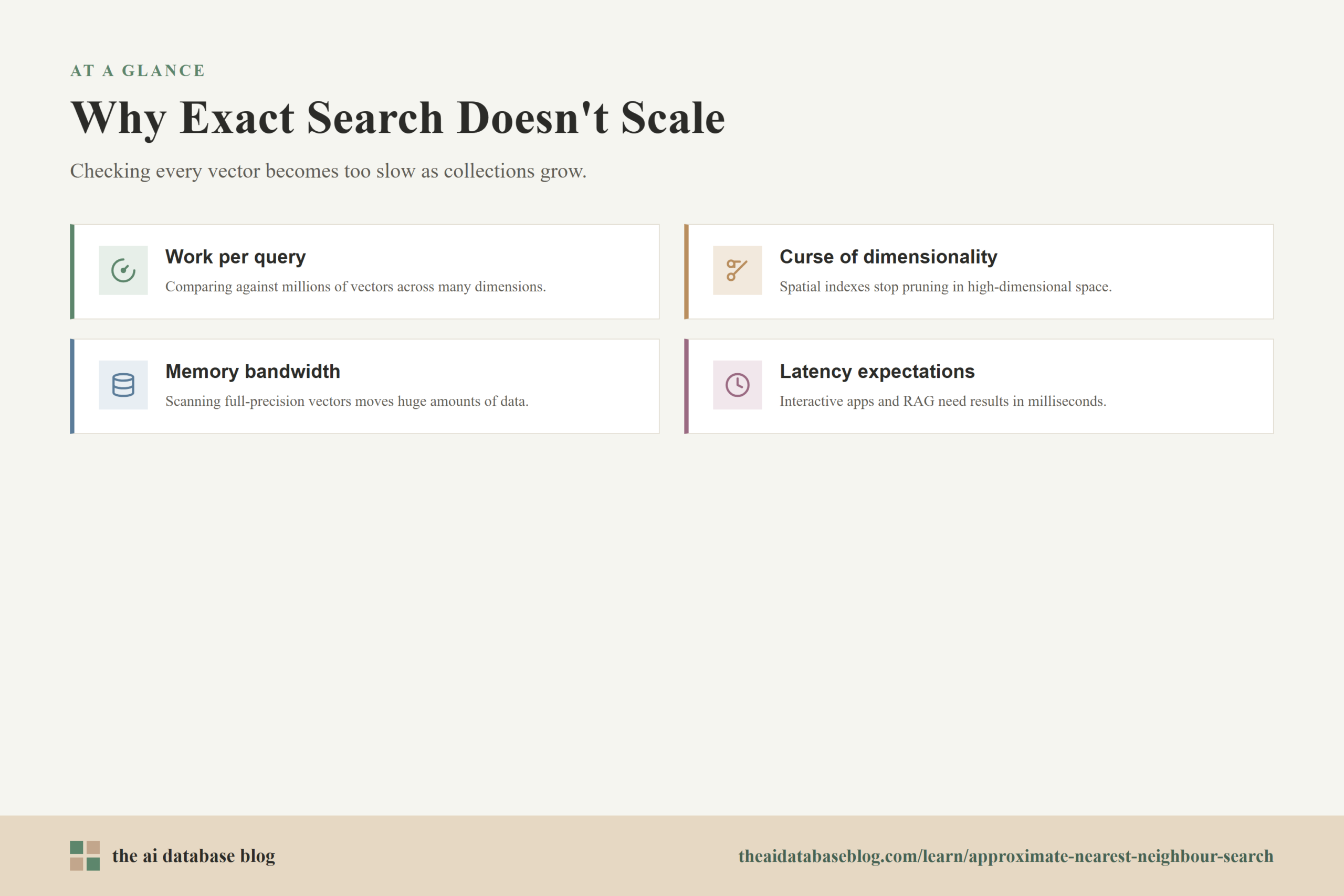
Exact search does not scale well because it has to do too much work per query. If a database contains 100 million vectors, exact search must compare the query vector against 100 million stored vectors unless another exact indexing structure can safely rule out candidates. Each comparison touches many dimensions, and the system still has to keep track of the best results. Even with optimized hardware, the cost grows with both the number of vectors and the size of each vector.
For low-dimensional data, traditional spatial indexes can sometimes reduce the search space effectively. In high-dimensional embedding spaces, those methods lose much of their advantage. Distances become harder to organize cleanly, partitions become less selective, and many points may look similarly far from the query. This is one practical form of the curse of dimensionality: structures that are efficient in two or three dimensions may stop pruning enough work when vectors have hundreds or thousands of dimensions.
Exact search also creates pressure on memory bandwidth. Vector comparison is not just a CPU problem; the system must load large amounts of vector data from memory or storage. A collection of float vectors can occupy substantial memory, and each query may require scanning enough data that memory movement becomes a bottleneck. If the system stores full-precision vectors for exact scoring, the storage and cache behavior can become as important as the distance formula itself.
Latency expectations make the problem sharper. Many AI applications need results fast enough to support an interactive user experience or a real-time model call. Retrieval-augmented generation, for example, often performs vector search before a language model response is generated. If retrieval adds hundreds of milliseconds or seconds under load, the whole application feels slow. Exact search may still be useful for small collections, offline evaluation, reranking small candidate sets, or workloads where correctness matters more than latency, but it is rarely the first choice for large interactive vector search.
The scaling problem leads directly to ANN search. If checking everything is too slow, the database needs a strategy for checking only the most promising areas of the collection while still returning results that are close enough to be useful.
What ANN Search Trades For Speed
ANN search speeds up vector retrieval by reducing the amount of work required for each query. Instead of proving that it has found the exact nearest neighbours, it uses an index structure that guides the search toward likely candidates. The result is usually much faster, but not guaranteed to contain every true nearest item. This is the core tradeoff: ANN search exchanges exactness for lower latency, higher throughput, and often lower operating cost.
The tradeoff is not a vague loss of quality. In most production systems, it is tunable. A graph index may search more neighbours before stopping. A clustering index may scan more clusters. A compressed index may rerank a larger candidate set using full-precision vectors. Increasing the search effort usually improves result quality and recall, but it also increases latency and resource usage. Reducing the effort makes queries faster, but it may miss more true neighbours.
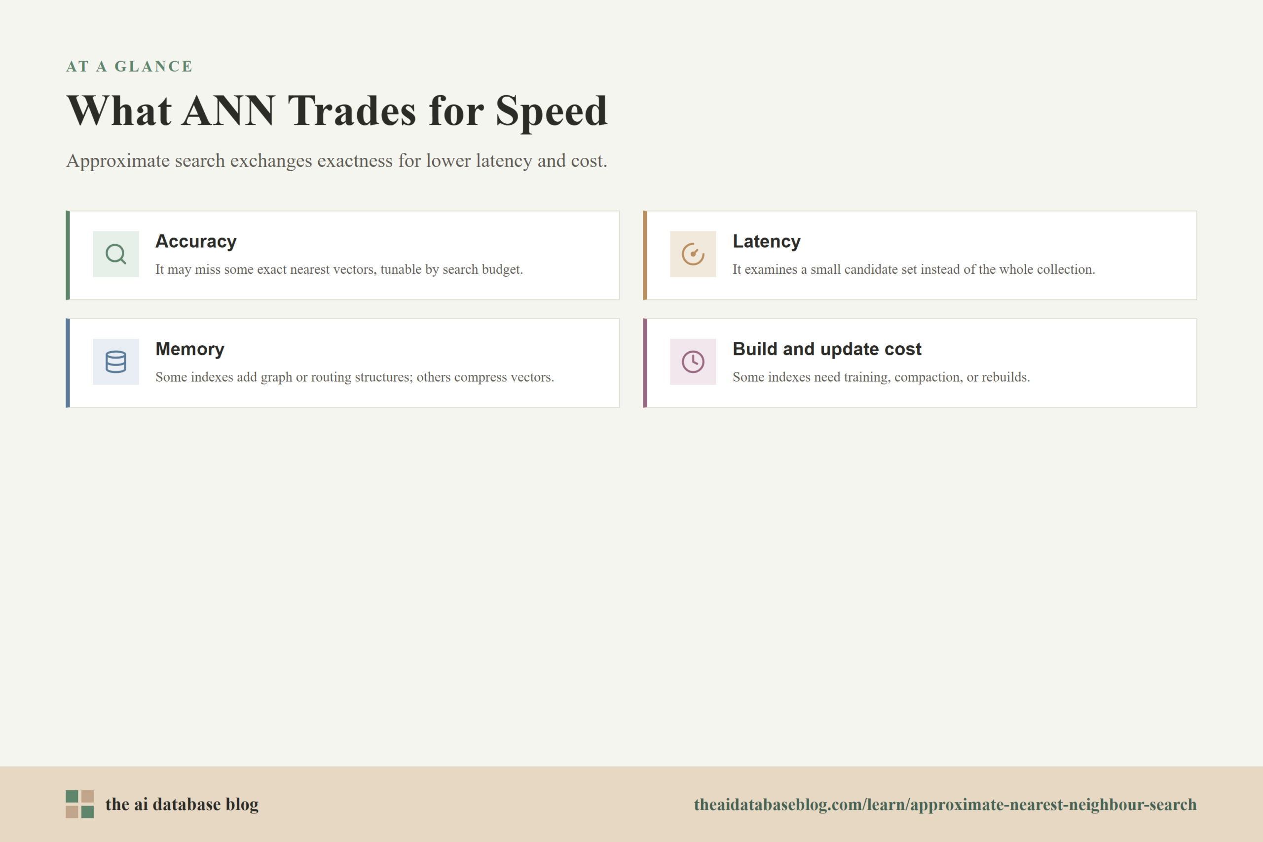
ANN systems commonly trade across four dimensions:
- Accuracy: The system may miss some of the exact nearest vectors, especially when the search budget is low or the data distribution is difficult.
- Latency: The system usually returns results much faster because it examines a small candidate set instead of scanning the full collection.
- Memory: Some indexes use extra memory for graph links, centroids, routing structures, or cached compressed representations. Others reduce memory by compressing vectors.
- Build and update cost: Some indexes are quick to build and easy to update. Others need training, careful construction, compaction, or rebuilding to keep search quality high.
These tradeoffs are why ANN search is not a single algorithm. It is a design space. Different indexes make different compromises, and real AI databases often combine techniques. A system might use clustering to narrow the search, product quantization to reduce memory, a graph to navigate candidates, and full-vector reranking to improve final quality.
Because ANN search deliberately gives up exact guarantees, teams need a practical way to talk about whether the results are good enough. That is where recall becomes central.
Recall Is The Key Quality Concept
Recall measures how many of the true nearest neighbours an ANN search returns. If exact search says the top 10 nearest vectors are A through J, and the ANN system returns 9 of those 10 somewhere in its top 10 results, the recall at 10 is 90 percent. In plain language, recall tells you how much of the exact answer set the approximate system managed to recover.
Recall is useful because it separates search quality from application quality. A retrieval system can fail because the embedding model is weak, the data is poorly chunked, the filters are wrong, the ranking logic is bad, or the ANN index missed relevant candidates. Recall focuses on the last issue: given the vectors and distance metric, did the index find the neighbours that exact search would have found?
Teams usually measure recall on a benchmark set. They choose representative query vectors, compute exact nearest neighbours as ground truth, run the ANN index, and compare the results. The key is to measure at the same result depth the application actually uses. Recall at 10, recall at 20, and recall at 100 can tell different stories. A RAG pipeline that retrieves 20 chunks before reranking should care about whether the right candidates appear in that candidate pool, not only whether the single closest vector is correct.
Recall should also be read alongside latency, throughput, memory, and filtering behavior. A system that reaches very high recall by spending much more time per query may not be suitable for an interactive product. A system that is fast on unfiltered benchmarks may behave differently when every query also includes tenant, permission, time, language, or category filters. In AI database work, recall is essential, but it is not the only metric that matters.
Once recall is understood, algorithm choices become easier to compare. The major ANN families differ mainly in how they decide which candidates are worth checking, how much memory they need, and how they let users tune the recall and speed balance.
A Map Of The Major ANN Algorithm Families
ANN algorithms can be grouped by the way they avoid exhaustive search. Some build a graph that lets the query move from candidate to candidate. Some partition the vector space into clusters and search only nearby partitions. Some compress vectors so that many approximate comparisons can be done cheaply. Some use hashing, trees, or disk-aware layouts. In practice, these families overlap, but the map is still useful because it explains the vocabulary used in vector database documentation and search benchmarks.
Graph-Based Indexes
Graph-based indexes connect vectors to nearby vectors, then search by navigating through the graph. The query starts from one or more entry points and moves toward candidates that appear closer. The search continues until the index has explored enough of the local neighbourhood to return likely nearest results. The best-known modern example is HNSW, which uses a hierarchy of graph layers to move quickly from broad navigation to fine-grained search.
Graph indexes are popular because they can achieve strong recall and low latency for many high-dimensional vector workloads. Their main cost is memory: the index must store graph connections in addition to vector data. They also expose important tuning parameters, such as how many neighbours each node keeps, how much effort is spent during construction, and how broadly the graph is explored during query time. Higher exploration usually improves recall but increases latency.
Inverted File And Cluster-Based Indexes
Inverted file indexes, often called IVF indexes, divide the vector collection into clusters. During index construction, the system learns representative centroids. Each stored vector is assigned to one or more nearby clusters. At query time, the system finds the closest centroids to the query and searches only the vectors in those selected clusters instead of scanning the full collection.
The main idea is search space reduction. If the query is near a few clusters, the system can ignore most other clusters for that query. The key tuning parameter is usually how many clusters are searched. Searching more clusters improves recall because the true neighbours are less likely to be missed, but it also increases latency. IVF approaches can work well for very large collections, especially when combined with compression or reranking.
Quantization And Compression Methods
Quantization methods reduce the memory and computation required to compare vectors. Product quantization, for example, breaks a vector into smaller parts and represents each part with a compact code. Instead of comparing full-precision vectors every time, the system can use compressed representations to estimate distances quickly. This is especially useful when vector collections are large enough that full-precision storage and scanning become expensive.
Compression introduces another kind of approximation. The system may not know the exact distance between the query and every stored vector from the compressed codes alone. To manage this, many systems use a two-stage process: first retrieve a candidate set using compressed or approximate distances, then rerank the best candidates with full-precision vectors. This pattern can reduce memory while preserving strong final result quality.
Hashing-Based Methods
Hashing-based ANN methods map similar vectors into the same or nearby buckets with high probability. Locality-sensitive hashing is the classic example. Instead of comparing the query to every vector, the system checks vectors in buckets that the query falls into. If the hash functions are well matched to the distance metric and data distribution, similar items are likely to become candidates.
Hashing can be conceptually simple and useful in some settings, but it is not always the strongest choice for modern high-recall embedding search. It may require many hash tables or careful tuning to get acceptable recall, and performance depends heavily on the data and metric. Still, hashing remains an important family because it shows one of the purest forms of ANN thinking: use probability to avoid looking everywhere.
Tree-Based And Space-Partitioning Methods
Tree-based methods organize vectors by recursively partitioning the space. In low-dimensional settings, trees can be very effective because a query can quickly rule out large regions. Examples include k-d trees and random projection trees. The challenge is that high-dimensional embeddings often weaken the pruning power of these structures, so the search may end up checking many branches anyway.
Tree-based methods still matter historically and can be useful for certain data shapes, lower-dimensional vectors, or as components in larger systems. They also help explain why ANN search evolved beyond traditional spatial indexing. Modern AI database workloads often need approaches that behave well when dimensionality is high, data is unevenly distributed, and query latency must remain predictable.
Disk-Aware And Hybrid Indexes
Disk-aware indexes are designed for collections that are too large or too expensive to keep entirely in memory. They use storage layouts, compressed in-memory summaries, graph navigation, and careful reranking to reduce the number of disk reads while still returning high-quality results. This family matters more as vector search moves into billion-scale and multi-tenant workloads where memory cost is a major constraint.
Hybrid indexes combine algorithmic ideas rather than treating them as separate choices. A system might use a graph for navigation, quantization for memory savings, full-precision reranking for quality, and filtering-aware execution for application constraints. This combination is increasingly common because real workloads rarely optimize only one variable. They need a working balance of recall, latency, memory, update behavior, and filtered search quality.
The algorithm map gives the main categories, but choosing among them depends on the workload. The same index can behave differently depending on collection size, vector dimensionality, update rate, filters, hardware, and the cost of missing a relevant result.
How ANN Search Fits Into An AI Database
In an AI database, ANN search is usually one part of a broader retrieval system. The database stores vectors, original objects, metadata, and sometimes multiple indexes over the same data. A query may include a vector similarity condition, keyword terms, metadata filters, access-control constraints, and a limit on how many results should be returned. The ANN index helps produce likely vector candidates, but the database still has to apply the rest of the query correctly.
This is why ANN behavior cannot be judged only from a pure vector benchmark. Real applications often use filters such as tenant ID, document type, language, region, date range, product availability, or user permissions. If the index retrieves approximate neighbours before filtering, it may return too few valid candidates after filters are applied. If filtering happens before vector search, the index needs a way to search efficiently inside the filtered subset. Different databases and index designs handle this problem differently.
ANN search also interacts with reranking. A common pattern is to retrieve a larger candidate set quickly, then apply a more expensive scoring step to a smaller group. The reranker might use exact vector distances, a cross-encoder, business rules, freshness signals, or a combination of features. In this architecture, the ANN index does not need to produce a perfect final ranking by itself. It needs to avoid missing candidates that the later stage would have ranked highly.
Updates are another practical concern. Some applications ingest data continuously, while others rebuild indexes in batches. Graph indexes, clustering indexes, and compressed indexes have different update costs and failure modes. A system that works well for a mostly static knowledge base may not be ideal for a stream of changing user events. Good ANN design starts with the retrieval workflow, not just the algorithm name.
With that context, the best way to evaluate ANN search is to connect index settings to application outcomes. The goal is not to maximize recall in isolation. The goal is to reach enough recall at an acceptable latency and cost for the specific retrieval task.
How To Think About ANN Settings In Practice
ANN settings control how hard the system works during indexing and querying. These settings often look different across databases and libraries, but they usually express the same idea: spend more resources to improve recall, or spend fewer resources to improve speed and cost. Understanding this pattern makes configuration less mysterious even when the parameter names vary.
For graph indexes, query-time settings often control how many candidate nodes the search explores before stopping. A higher value usually means the search has more chances to find the true nearest neighbours. Construction settings may control how dense the graph is or how carefully links are selected. A denser or more carefully built graph can improve recall, but it may use more memory and take longer to build.
For IVF-style indexes, settings often control the number of clusters and the number of clusters searched per query. Too few clusters can make each cluster large, reducing the benefit of partitioning. Too many clusters can make training and assignment more complex. Searching more clusters usually improves recall but increases the number of vectors examined. The right balance depends on the collection size and data distribution.
For quantized indexes, settings control compression strength and reranking depth. More aggressive compression can reduce memory and speed up candidate generation, but it may distort distances. Reranking more candidates with full-precision vectors can recover quality, but it adds work. This is a common and useful pattern: approximate broadly, then score a smaller set more accurately.
Practical tuning should use representative data and queries. A configuration that looks good on random test vectors may not work for real user questions, filtered searches, or long-tail content. The most useful evaluation combines recall against exact ground truth, latency under realistic load, memory use, update behavior, and final application quality. For RAG, that may include whether the retrieved context actually helps answer questions. For recommendations, it may include engagement or relevance metrics. For deduplication, it may include false positives and false negatives.
These practical choices bring the discussion back to the central point: ANN is not about accepting bad search. It is about spending the search budget where it matters most.
Common Use Cases For ANN Search
ANN search is useful when an application needs similarity search over enough vectors that exact search is too slow or too costly. The most familiar use case is semantic search, where users search by meaning instead of exact words. A support knowledge base, documentation site, or internal policy library can embed passages and use ANN search to retrieve the most relevant ones for a natural-language query.
Retrieval-augmented generation is another major use case. In a RAG system, ANN search finds candidate chunks that may contain information needed by a language model. The system may then rerank or filter those chunks before adding them to the model context. Here, recall matters because missing the right passage can lead to incomplete or incorrect answers even if the model itself is capable.
Recommendation systems also rely on nearest neighbour patterns. A user, product, article, or media item can be represented as an embedding, and ANN search can quickly find similar items or candidate recommendations. The ANN stage often produces a broad candidate set, while later ranking stages personalize, diversify, or apply business constraints.
Other use cases include image similarity, duplicate detection, anomaly investigation, entity resolution, and clustering large collections. In each case, ANN search helps the system avoid exhaustive comparison while still surfacing nearby items. The value comes from matching the algorithm and settings to the tolerance for missed neighbours, the size of the data, and the latency expectations of the product.
These use cases differ, but they share a practical pattern: exact search defines the ideal neighbour set, ANN search makes retrieval feasible at scale, and evaluation determines whether the approximation is good enough for the job.
FAQs
1. What is approximate nearest neighbour search?
Approximate nearest neighbour search is a way to find vectors that are very close to a query vector without checking every stored vector exactly. It uses an index to guide the search toward likely candidates, which makes retrieval much faster at large scale. The result is approximate because the system may miss some of the exact nearest neighbours, depending on the index and settings.
2. Why not always use exact vector search?
Exact vector search is simple and accurate, but it becomes expensive when collections contain millions or billions of high-dimensional vectors. Each query may require a large number of distance calculations and a large amount of memory access. Exact search is still useful for small datasets, offline ground-truth evaluation, and reranking small candidate sets, but ANN search is usually more practical for large interactive AI applications.
3. What does ANN search trade for speed?
ANN search trades guaranteed exactness for speed, throughput, and sometimes lower memory or storage cost. It does this by searching only promising candidates instead of the whole collection, or by using compressed representations before final scoring. The tradeoff can usually be tuned: more search effort improves recall, while less effort improves latency.
4. What is recall in ANN search?
Recall measures how many true nearest neighbours the approximate search returns. If exact search identifies 10 correct nearest neighbours and the ANN index returns 9 of them in its top 10 results, recall at 10 is 90 percent. Recall is important because it helps teams quantify how much quality they are giving up for speed.
5. Which ANN algorithm family is best?
There is no single best ANN algorithm family for every workload. Graph-based indexes often offer strong recall and latency but can use more memory. IVF-style indexes reduce the search space through clustering and can work well at large scale. Quantization reduces memory and comparison cost. Disk-aware and hybrid approaches matter when collections are very large or memory cost is a constraint. The best choice depends on data size, latency goals, filters, update patterns, and required recall.
6. How should teams evaluate ANN search for RAG?
Teams should evaluate ANN search for RAG by measuring recall against exact nearest neighbours, latency under realistic load, and the quality of the final retrieved context. It is important to test with real queries, real chunks, and real filters because synthetic benchmarks may not show how the system behaves in production. A useful ANN configuration is one that retrieves enough relevant candidates for the reranker or language model while staying within the application’s latency and cost limits.
Takeaway
Approximate nearest neighbour search is the practical foundation of large-scale vector retrieval in AI databases. Exact search gives the clean mathematical answer, but it often becomes too slow and resource-heavy for high-dimensional embedding collections. ANN search makes the problem workable by navigating, partitioning, compressing, hashing, or otherwise narrowing the candidate set, with recall used to measure how much of the exact answer it still captures. This guidance is most useful for engineers, technical content teams, and product builders who need to understand how vector search behaves in semantic search, RAG, recommendation, and similarity-driven applications.